Level up your Excel skills and unlock the power of data visualisation with conditional formatting. This course will take you from basic formatting to advanced data analysis techniques to change the way you work with spreadsheets.
by Mihir Kamdar / Last Updated:
In this course you’ll learn:
Basic conditional formatting techniques for data analysis and how to use conditional formatting to highlight cells based on their content
The versatility of conditional formats, including how to apply multiple rules to the same cells based on specific business logic
Advanced formula based comparison
How to create professional visualisations with Data Bars, Color Scales and Icon Sets
Download our step-by-step tutorial file now by clicking on the icon below and follow along to enhance your Excel skills practically and efficiently!
Excel’s conditional formatting is a game changer that turns messy data into clear insights. Whether you’re a business analyst, financial professional or data geek, mastering conditional formatting will change the way you analyse and present data. This course will take you from the basics to advanced techniques to create dynamic, visually appealing spreadsheets that communicate your findings.
Understanding how to use conditional formatting in Excel is essential for making data stand out and improving overall readability. With Excel: Conditional Formatting, users can apply dynamic rules to their data, such as highlighting cells based on specific conditions. The formula for conditional formatting Excel allows for detailed customization, enabling you to tailor your formatting to fit complex scenarios. For instance, formatting cells Excel can be done using data bars, color scales, or icon sets, which visually represent values effectively.
If you’re wondering where is conditional formatting in Excel, it can be found in the “Home” tab under the “Styles” group. From there, you can create rules using a conditional format formula Excel or choose from predefined settings. To apply this feature effectively, learning about conditional formatting with examples is vital. For instance, highlighting overdue tasks or sales figures exceeding targets demonstrates how to use conditional formatting on Excel for practical applications.
When dealing with outdated styles, knowing how to clear formatting in Excel is important. You can do this by selecting the range and choosing the “Clear Rules” option, which ensures a clean slate for new rules. Similarly, how to remove formatting in Excel is straightforward and helps maintain a neat dataset. For users exploring advanced techniques, conditional formatting Excel formula and formula Excel conditional formatting offer powerful tools for complex data comparisons.
Understanding what is conditional formatting in Excel opens up opportunities to enhance your reports. Whether it’s using Excel formatting to create professional dashboards or format conditional formatting to highlight specific trends, the possibilities are extensive. By mastering these techniques, you can transform raw data into actionable insights, making spreadsheets not only functional but visually engaging.
Conditionally format is a powerful Excel feature that turns messy data into meaningful insights. This feature automatically formats cells based on certain conditions so you can easily see patterns, trends and outliers in your data.
Benefits:
See trends and patterns in large datasets quickly
Highlight important data automatically
Create professional looking reports and dashboards
Improve data visualisation and presentation
Save time on manual formatting
Highlight duplicate values
Conditional formatting is a powerful feature in Excel that allows you to highlight cells based on specific conditions, such as values, formulas, or formatting. This feature enables you to visually differentiate your data, making it easier to analyze and understand. By applying conditional formatting, you can change the background color, font color, or border style of cells that meet certain criteria. This not only enhances the visual appeal of your spreadsheets but also helps in quickly identifying key data points, trends, and outliers.
Conditional formatting Excel is a powerful tool to enhance data visualization and analysis. Excel conditional formatting allows users to highlight data trends and patterns by applying formatting rules. Conditional formatting in Excel simplifies large datasets by emphasizing key values, trends, or outliers.
Excel conditional formatting and its features, such as data bars and color scales, are widely used for professional reporting. If you’re wondering how to do conditional formatting in Excel, simply follow the steps to apply rules based on conditions or formulas. Excel conditional formatting formula options enable advanced customizations, such as highlighting specific orders or applying rules dynamically.
Clearing formatting in excel, use the “Clear Rules” option under the conditional formatting menu. Excel clear formatting and clearing formatting in Excel help remove unwanted or outdated rules to tidy up your spreadsheets. Xls conditional formatting is especially beneficial for older Excel versions, ensuring compatibility. For tasks like conditional formatting to highlight specific orders Excel offers a variety of formulas to suit diverse needs. Understanding conditional formatting and mastering these techniques will undoubtedly elevate your spreadsheet skills.
Applying conditional formatting in Excel involves a few simple steps. Here’s how you can do it:
Select the cells you want to format.
Go to the Home tab in the Excel ribbon.
Click on the Conditional Formatting button in the Styles group.
From the dropdown menu, select the type of formatting rule you want to apply.
Enter the condition or formula that you want to use to determine which cells to format.
Choose the format you want to apply to the cells that meet the condition.
Click OK to apply the formatting rule.
By following these steps, you can apply conditional formatting to highlight important data points and make your spreadsheets more informative.
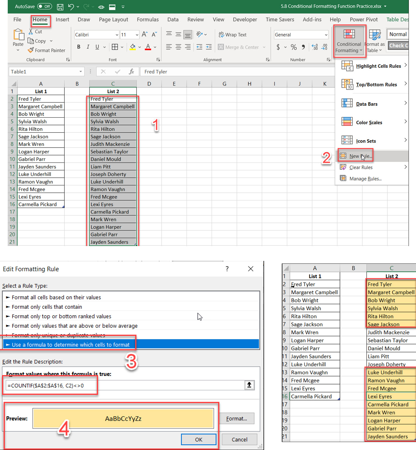
This technique matches values between two lists using conditional formatting functions.
Steps:
Select the criteria data (C2:C21)
Go to Home → Conditional formatting → New rule
Click on “Use a formula to determine which cells to format” and enter the formula: =COUNTIF($A$2:$A$16, C2)< > 0
Click conditional formatting to apply the rule
$A$2:$A$16 is the criteria range (where it will search for criteria, C2 is the criteria)
The range selected in step 1 (C2:C21) will loop through $A$2:$A$16
Your criteria range must be an absolute reference
< >0 means data in both lists match

Pro Tips for List Comparison:
Use this for inventory reconciliation
Compare customer lists across different periods
Find matching transactions in financial data
Validate data across worksheets
This is for data validation and error checking.
Steps:
Select the data range (C2:C21)
Go to Home → Conditional formatting → New rule
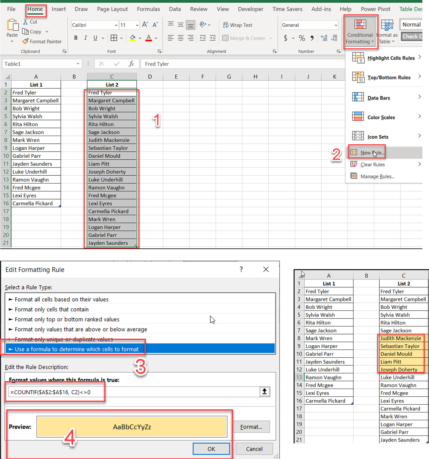
Click “Use a formula to determine which cells to format” and enter: =COUNTIF($A$2:$A$16, C2)=0
To clear rules from selected cells, go to Home → Conditional formatting → Clear Rules → Clear Rules from Selected Cells
Formula explanation same as above, but =0 means non-matches

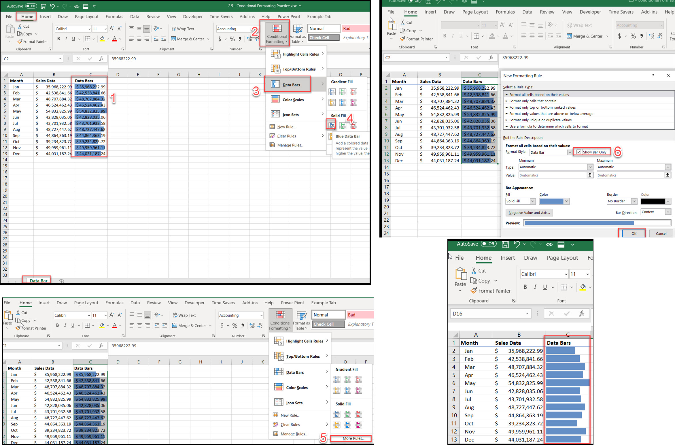
Data Bars applies colors and bars to cell values, instant visual impact.
Steps:
Select cells
Home → Conditional Formatting → Data Bars
Choose your color scheme
Optional: Select “More Rules” to customize
Consider “Show Bar Only” for a cleaner look

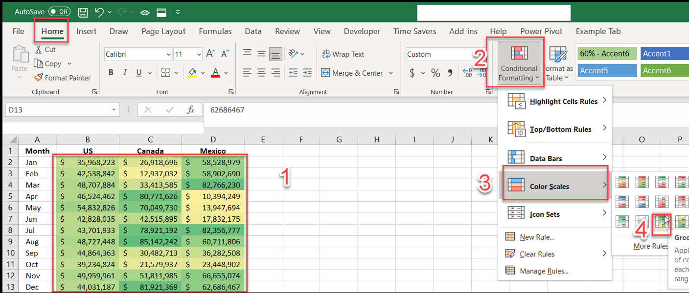
Color Scales applies background colors to cell values, heat map style.
Steps:
Select cells
Home → Conditional Formatting → Color Scales
Choose your color scheme

Icon Sets applies visual indicators to cell values, great for status and KPI reporting.
Steps:
Select cells
Home → Conditional Formatting → Icon Sets
Choose your icon theme
For more specific criteria, use Highlight Cells Rules to apply conditional formatting based on values or text.
Conditional formatting is a feature in Excel that automatically applies formatting to cells based on specific conditions or rules. It allows you to highlight important data, identify trends, and make your spreadsheets more visually appealing and easier to analyze.
To apply conditional formatting:
Select the cells you want to format
Go to the Home tab and click on Conditional Formatting
Choose a rule type (e.g., Highlight Cells Rules, Top/Bottom Rules)
Set the condition and choose the formatting style
Click OK to apply the formatting
Yes, you can apply multiple rules to the same cells. However, it’s important to arrange the rules in the correct order of priority using the Rules Manager to ensure they work as intended.
To edit or delete rules:
Select the cells with conditional formatting
Go to Conditional Formatting > Manage Rules
In the Rules Manager, select the rule you want to edit or delete
Click Edit Rule to modify it, or use the Delete Rule button to remove it
Yes, you can create conditional formatting rules based on the values in other cells. This is often done using formulas in the conditional formatting rule.
You can copy conditional formatting using two main methods:
Simple copy and paste
Using the Format Painter tool in the Home tab
Excel offers various types of conditional formatting, including:
Highlight Cells Rules (e.g., greater than, less than, equal to)
Top/Bottom Rules
Data Bars
Color Scales
Icon Sets
Custom formulas
To apply conditional formatting, go to the Home tab, then click Conditional Formatting in the Styles group. Choose a rule type or create a custom rule to highlight important data visually based on specific conditions.
Mastering Excel’s conditional formatting transforms your ability to analyze and present data effectively. By applying these techniques, you’ll create powerful visual insights that enhance decision-making and communicate complex data clearly. Remember to practice with the provided exercise files and experiment with different combinations of formatting rules to find what works best for your specific needs.
To format your data efficiently, click Highlight Cells Rules under the Conditional Formatting dropdown and choose a specific condition for your dataset. Use absolute cell references in your formulas when applying a conditional format to ensure consistent results across your Excel sheet. Open the formatting rule dialog box in Excel to define specific criteria for highlighting only cells that meet your chosen conditions. Excel allows you to click Highlight Cells Rules and use formulas with absolute cell references to create customized conditional format rules for your data.

92% of students automate workflows, build CEO-ready dashboards, and streamline collaboration in < 1 hour. Don’t miss out!
🎯Master every Office 365 tool like Excel, Word, PowerPoint, Teams, Outlook and OneNote.
🎯Streamlined approach—no fluff, just rapid skill-building.
🎯Eliminate tedious tasks with intelligent automation.
🎯Transform everyday workflows into strategic power moves.
🎯Boost productivity and impress every boss.
🎯Real-World Projects – directly translate lessons into workplace wins.