Learn how to create a drop down list in Excel with this guide. Get step-by-step instructions, tips, and best practices to make effective and dynamic drop down menus in Excel for fast data entry and increased productivity. Excel has a data validation tool ti create drop down list.
by Mihir Kamdar / Last Updated:

After reading this guide, you’ll be equipped with the knowledge to:
Download our step-by-step excel file now by clicking on the icon below and follow along to enhance your Excel skills practically and efficiently!
Dropdowns are powerful tools for choosing from a list of options in a cell. They are super useful for data consistency, reducing errors, and making spreadsheets more user-friendly. Whether you’re managing inventory, tracking projects, or creating forms, knowing how to make a dropdown list will take your Excel skills to the next level.
A drop down list is a feature that allows you to choose a value from a list of options in a cell. This is done using Excel’s Data Validation feature, so only specified values are allowed in a cell, and data is kept consistent and clean.
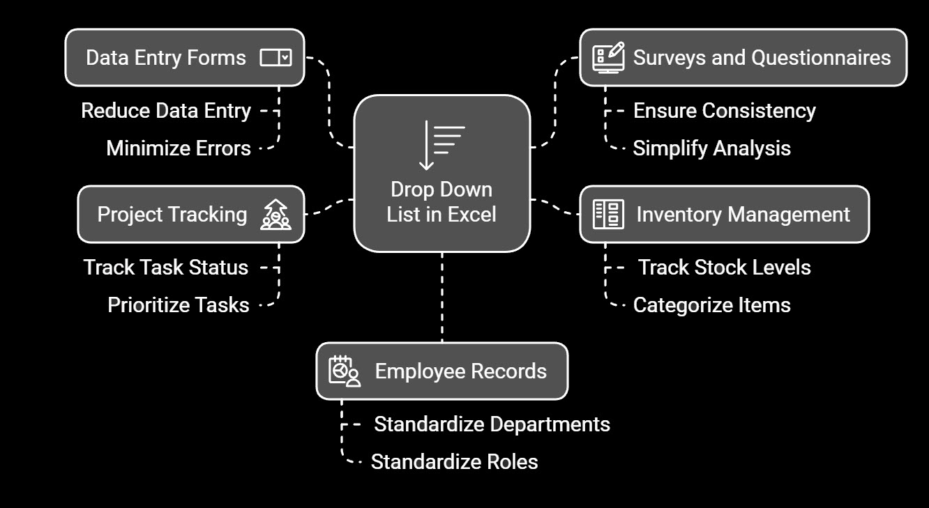
Drop Down List Examples:
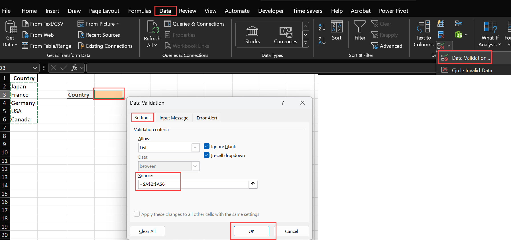
Select the Cell: Click on the cell where you want the drop-down to appear.
Select Data Validation: Go to the Data tab on the ribbon > Click on Data Validation in the Data Tools group.
Set the List Source:
Input Messages and Error Alerts (Optional):
Click OK: Your drop-down is now in the cell.
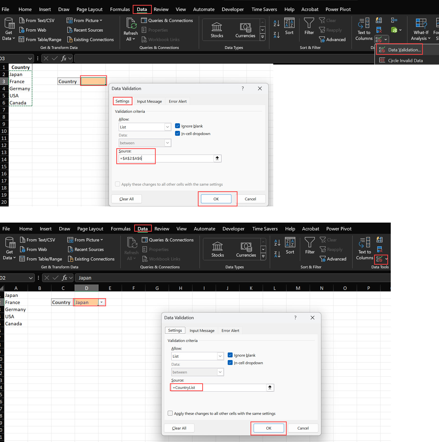
Dynamic drop-down lists update as you add or remove items from the source list. This is handy when you want to keep the options up to date without manually changing the Data Validation settings.
Create a Named Range:
Apply Data Validation:
=OptionsList in the Source field.Update the List:
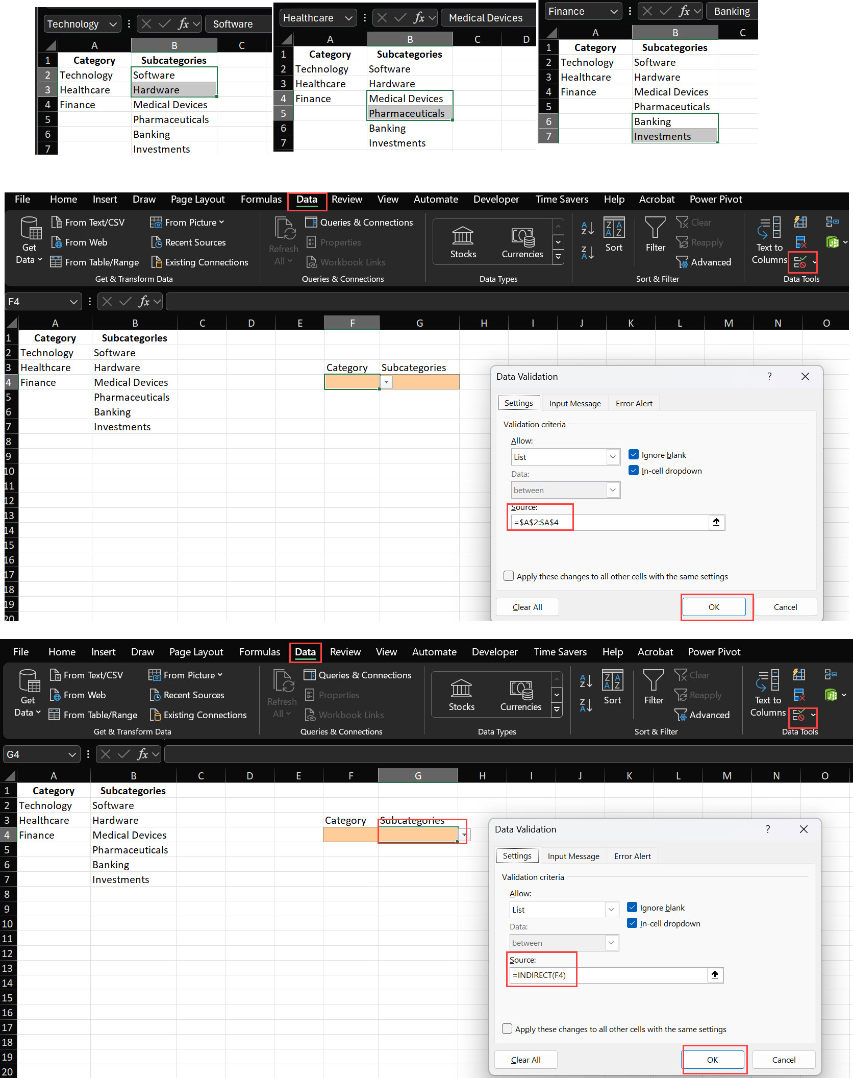
Dependent drop-downs, also known as cascading drop-downs, change their options based on the selection made in another drop-down. This is useful for hierarchical data selection, for example, choosing a category first and then a subcategory.
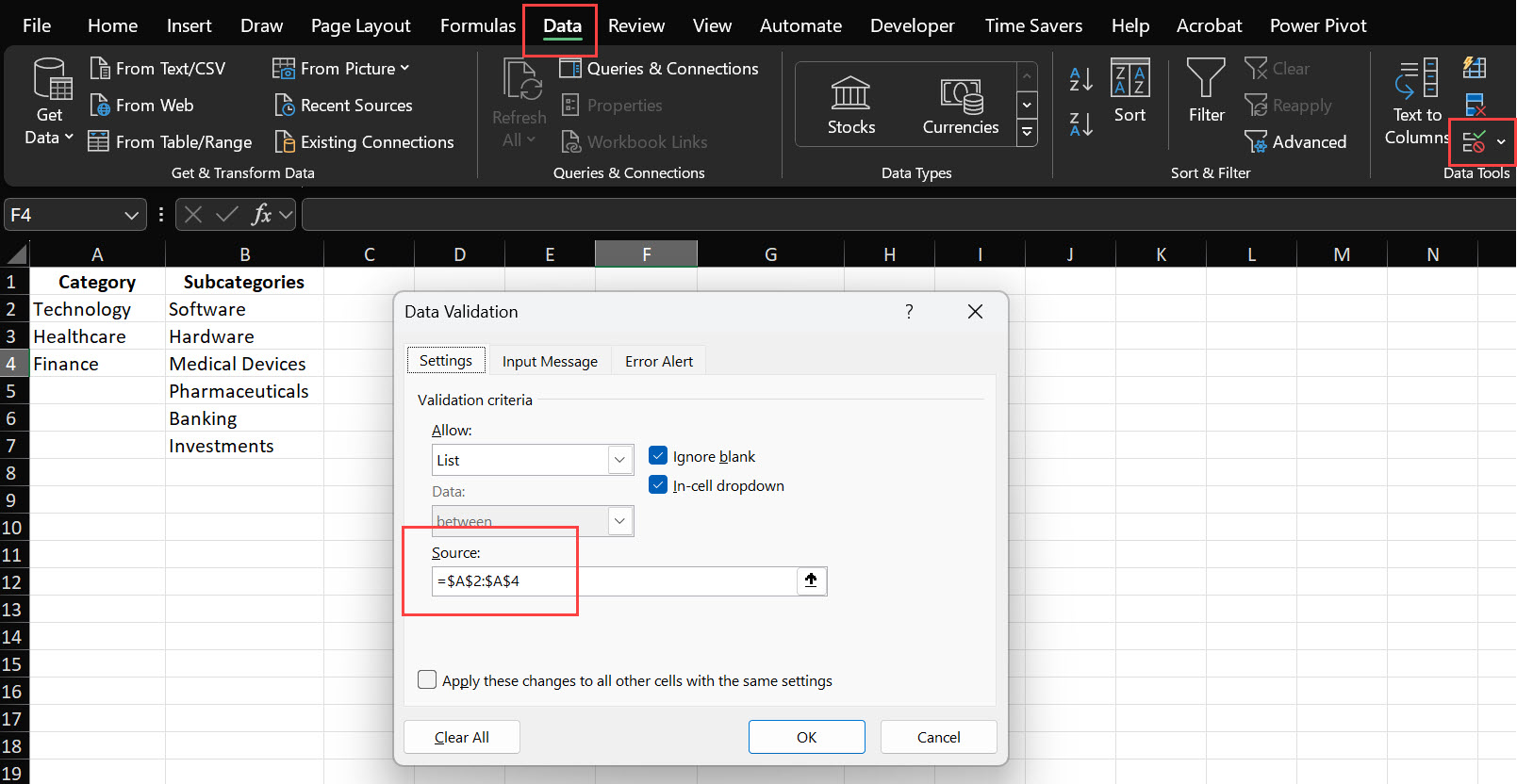
Create Primary and Secondary Lists: For example, create a list of categories in A2:A3 and subcategories in B2:B7.
Name Your Ranges: Select the subcategories for each category and name the range the same as the category.
Apply Data Validation for Primary List: Select the primary cell and apply Data Validation with the primary list.
Apply Data Validation for Secondary List: Select the secondary cell, and in the Source field, type =INDIRECT(A1) where A1 is the cell with the primary drop-down.
Click OK: The secondary drop-down will now show options based on the primary selection.
To edit the items in your dropdown:
Select the Cell with the Dropdown: Click on the cell with the dropdown.
Go to Data Validation: Go to Data > Data Validation.
Edit the Source: Edit the list items in the Source field or update the range.
Click OK: The dropdown will update.
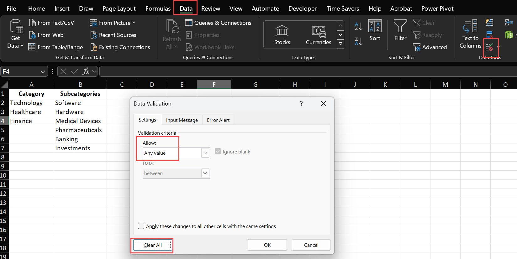
To remove a dropdown from a cell:
Select the Cell: Click on the cell with the dropdown.
Go to Data Validation: Go to Data > Data Validation.
Clear All: Click Clear All in the Settings tab.
Click OK: The dropdown is removed and the cell is now blank.
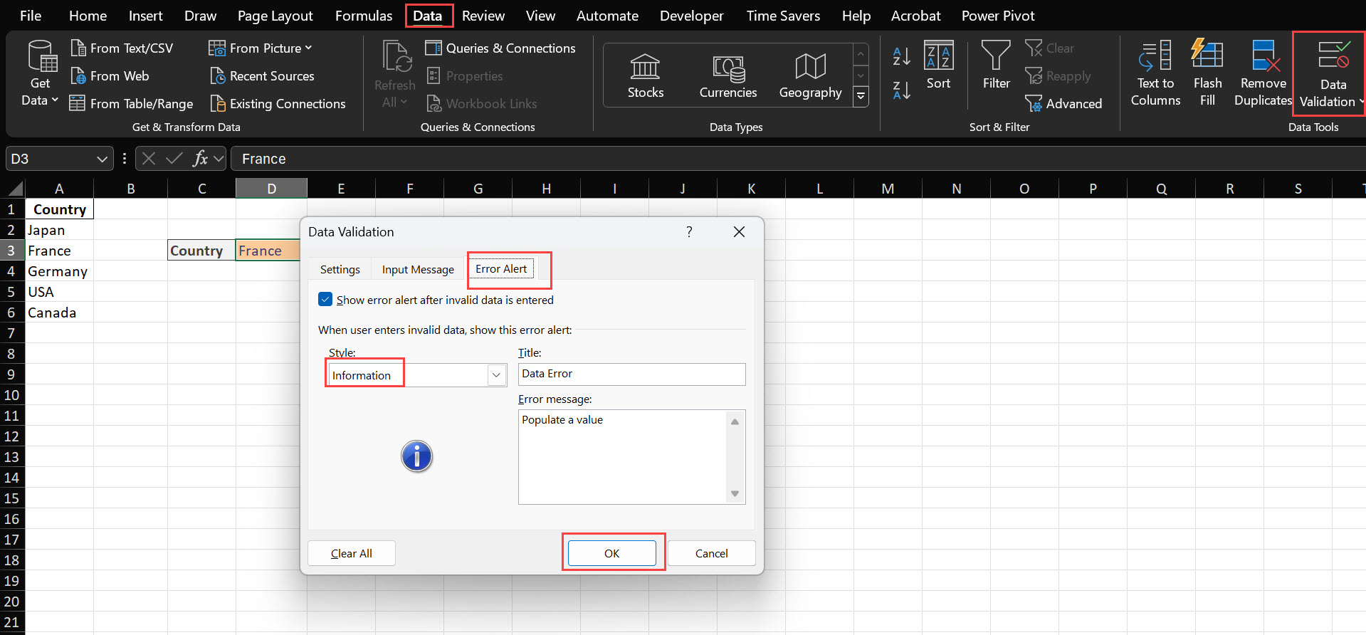
Excel’s Data Validation feature allows you to control what happens when a user enters invalid data that does not meet the rules you’ve set. This helps maintain the integrity of your data and guides users to input correct values.
Open the Data Validation Settings:
Navigate to the Error Alert Tab:
Set Up Your Error Alert:
Configure the Alert Options:
Save Your Settings:
Data Consistency: Don’t duplicate entries and standardize list items to be uniform.
Performance: For large lists use dynamic ranges or tables to keep performance fast.
User Experience: Keep dropdowns short and relevant and provide instructions or labels for the user.
Named Ranges: Simplify formula management and make it more readable by using descriptive named ranges.
Update Lists Regularly: Keep your dropdowns up to date by regularly reviewing and updating the source data.
Limit List Length: For usability, keep dropdowns to a reasonable length to not overwhelm the user.

Use Data Validation to create drop down lists:
Select the cell.
Go to Data > Data Validation.
Select List from the Allow dropdown.
Type in your list items or select a range with the items.
Click OK.
Yes, you can have multiple dependent (cascading) dropdowns in Excel by using named ranges and the INDIRECT function to set up primary and secondary dropdowns. This will make the options in one dropdown depend on the selection in another.
Make a dropdown dynamic by using named ranges that expand with new items or by converting your list data into Excel tables. This will make your dropdown update automatically when new items are added or removed.
Creating a dropdown in Excel is a basic skill that will help you manage your data, ensure consistency, and improve user experience. Whether you use basic Data Validation, dynamic named ranges, or advanced VBA scripts, you’ll be more productive and your spreadsheets will be more user-friendly.

92% of students automate workflows, build CEO-ready dashboards, and streamline collaboration in < 1 hour. Don’t miss out!
🎯Master every Office 365 tool like Excel, Word, PowerPoint, Teams, Outlook and OneNote.
🎯Streamlined approach—no fluff, just rapid skill-building.
🎯Eliminate tedious tasks with intelligent automation.
🎯Transform everyday workflows into strategic power moves.
🎯Boost productivity and impress every boss.
🎯Real-World Projects – directly translate lessons into workplace wins.