Discover how to transform your boring spreadsheets into professional, eye-catching documents with these 6 essential Excel formatting tricks. Learn time-saving shortcuts, data visualization techniques, and pro tips to enhance your spreadsheet skills and impress your colleagues.
by Mihir Kamdar / Last Updated:

After reading this guide, you’ll be equipped with the knowledge to:
Quick number formatting techniques for financial data
How to use conditional formatting for data analysis
Creating and managing dynamic Excel tables
Applying professional cell styles and custom formatting
Text alignment secrets for better readability
Using borders to organize and separate data effectively
Download our step-by-step tutorial file now by clicking on the icon below and follow along to enhance your Excel skills practically and efficiently!
Let’s face it – staring at rows and columns of raw data is about as exciting as watching paint dry. But what if I told you that with a few simple tricks, you could turn those mind-numbing spreadsheets into sleek, professional documents that actually make sense? In this guide, we’ll dive into six game-changing Excel formatting hacks that’ll have you looking like a spreadsheet wizard in no time. Whether you’re a number-crunching newbie or a seasoned Excel veteran, these tips will help you work smarter, not harder.
If you’re working with Excel, knowing how to clear formatting in excel is a must for tidying up your spreadsheets. To excel quickly format sheet, you can use pre-designed templates or the format painter tool. If you’re wondering how to get excel to save formatting, ensure you’re saving the workbook properly to retain styles and adjustments.
The excel format options provide a range of features, including number, text, and date formatting, along with excel table formatting for creating visually appealing tables. For specific edits, understanding how do you format excel cells can help you customize borders, fill colors, and more. Learning excel tricks, like using shortcuts, speeds up your workflow significantly.
You can also explore how to format an excel cell to set data types, while advanced users may need to change the excel document format when saving files in different formats like .xlsx or .csv. Knowing how to remove formatting in excel is essential for reverting cells to default settings without deleting content, and excel formatting options make this a breeze.
Additionally, mastering the excel ‘format’ options and the excel format painter keyboard shortcut helps you copy styles efficiently across your workbook.
To ensure proper formatting in Excel, it’s important to modify selected cells without impacting adjacent ones. If a value is displayed incorrectly, it’s likely due to formatting and not the value itself. Using the select format cells option, you can apply predefined formats like dates, numbers, or text for consistency. For financial data, set the default currency symbol to match your region, ensuring accuracy and readability. These steps help create polished and professional-looking spreadsheets.
To make your Excel spreadsheets more professional and efficient, focus on formatting techniques like adjusting the font size and font color to improve readability and design. Utilize features to highlight filter and sort for easy data management. Advanced tools like “Copilot” allow you to sort data with Copilot automatically, streamlining tasks. You can also manually filter and sort data using Excel’s built-in options for quick categorization and analysis. These methods enhance your workflow and make data visually appealing and organized.
To improve the appearance and functionality of your Excel sheets, focus on effectively managing cell contents to present clear data. You can effortlessly highlight filter options to locate and organize information quickly. Additionally, use customizable border styles to separate and define sections of your spreadsheet, making it more organized and professional.
Mastering Excel requires understanding basic concepts such as excel 101, which covers the essentials for beginners. Knowing the excel workbook format is critical for managing and saving your files properly. If you need to tidy up data, learning to clear format in excel ensures your sheets are clean and organized. Various excel formats are available for numbers, dates, and text, each offering tailored customization.
To speed up formatting tasks, the excel format painter shortcut keyboard is invaluable for replicating styles. The excel doc format allows you to save your work in multiple file types like .xlsx or .csv for compatibility. You may need to learn how to format cells excel to apply styles, colors, or alignment effectively. For creating polished sheets, understanding how to format excel sheet helps streamline your layout.
Excel offers many advanced tools, including total cell style excel options for pre-designed layouts and tips en excel to improve productivity. Keyboard shortcuts like the format painter excel shortcut key make formatting tasks faster, while exploring format excel cells ensures professional-looking sheets. If you’re new to advanced customization, how to format in excel provides insights into text and numerical formatting.
Understanding how to clear table formatting in excel is vital for resetting tables, and excel formatting in formula allows you to integrate formatting within calculations. Knowledge of formula format in excel improves how data is presented. Whether you’re focusing on format excel tasks or cell formatting in excel, these tips ensure your spreadsheets stand out.
Lastly, techniques for formatting excel spreadsheets give you a structured, visually appealing document that’s easy to read and share.
Ever seen a financial report where the numbers look like they’ve been tossed in a blender? Yeah, not cool. Using custom formats can help you display values dynamically and intuitively. Consistent number formatting is the secret sauce to making your data look pro. Implementing a custom number format allows you to make numerical values visually descriptive while keeping them suitable for calculations.
How to Nail It
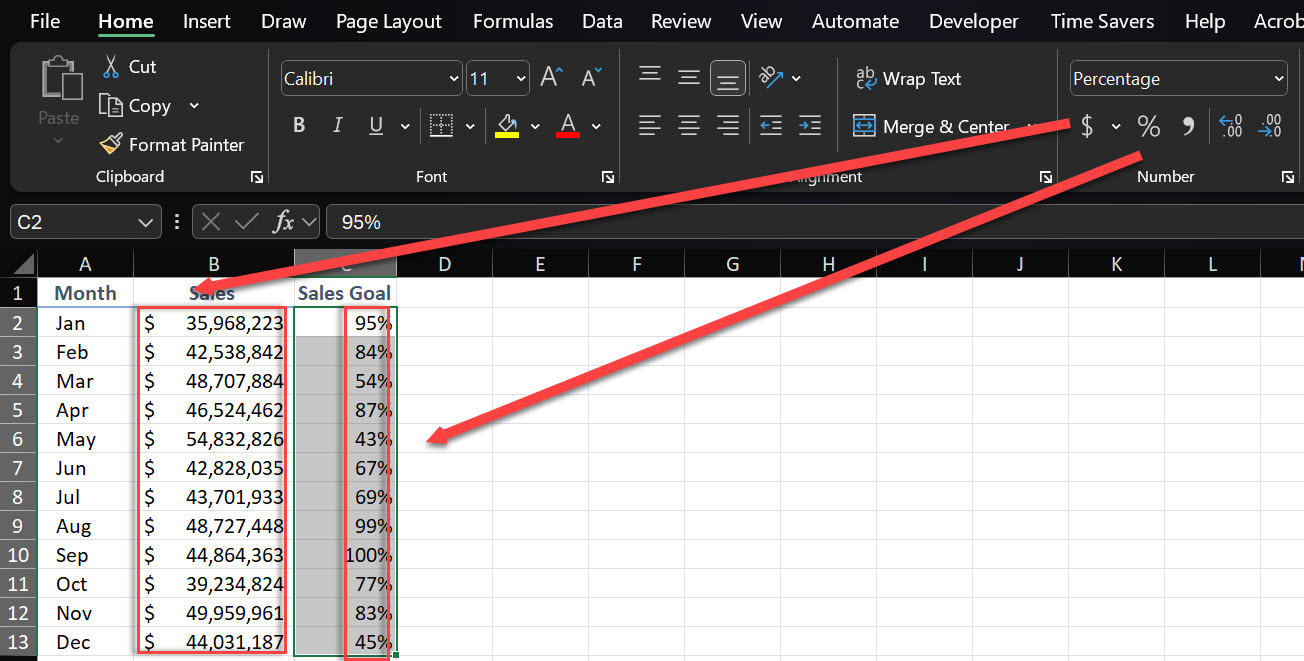
For instant currency formatting: Highlight your cells and hit Ctrl + Shift + $.
To turn those decimals into percentages: Select and press Ctrl + Shift + %.
Want to make important data pop without manually highlighting every cell? Conditional formatting is your new best friend.
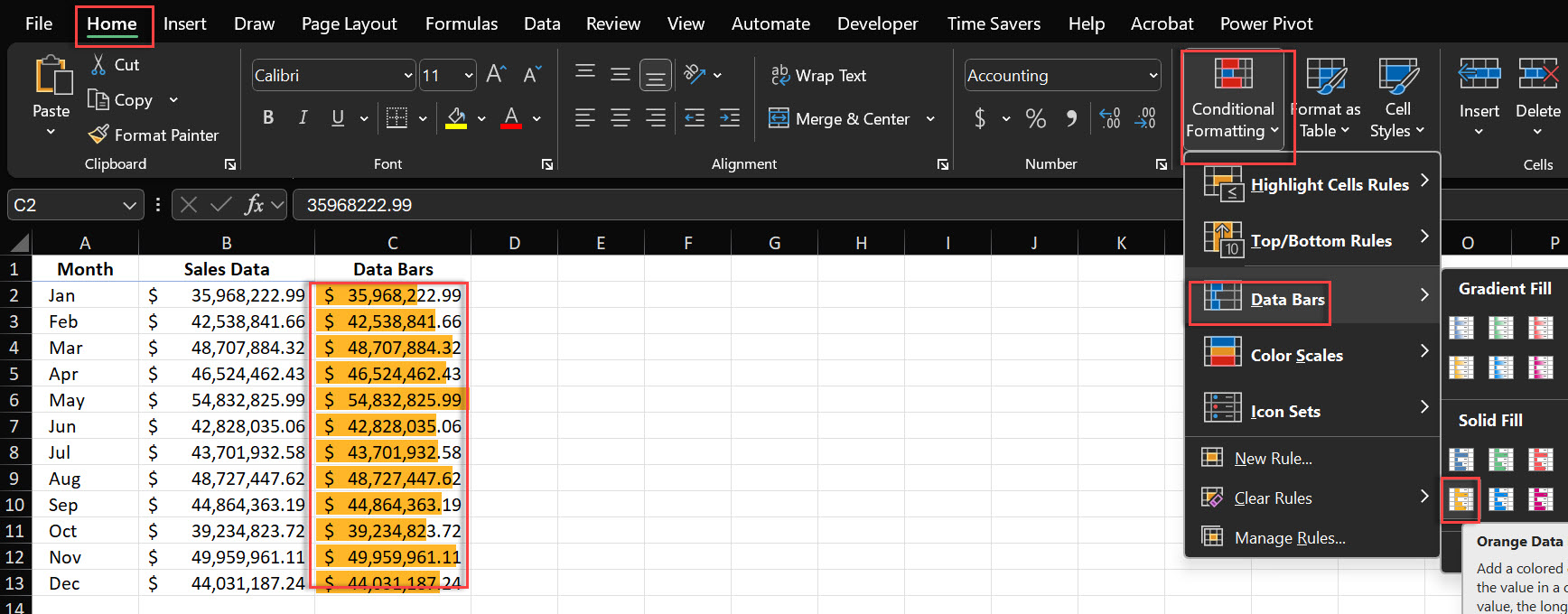
Data Bars
Select your data range.
Head to Home > Conditional Formatting.
Choose from Data Bars.
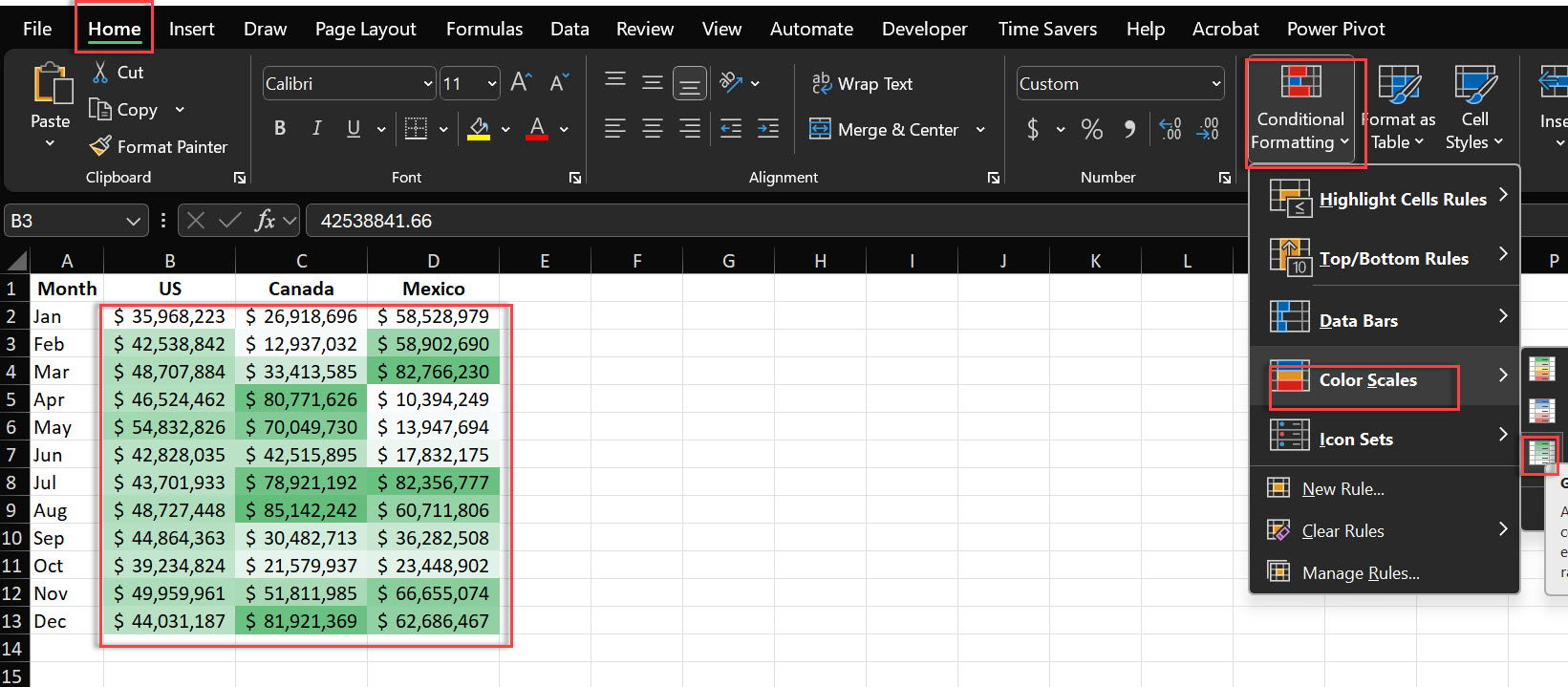
Color Scales
Select your data range.
Head to Home > Conditional Formatting.
Choose from Color Scales.
Pro tip: Use color scales to create a heat map of your sales performance across different regions. High performers will stand out in green, while areas needing attention will show in red.
Icon Sets
Select your data range.
Head to Home > Conditional Formatting.
Choose from Icon Sets
Say goodbye to manual updates and hello to dynamic tables that grow with your data.
The Magic Trick
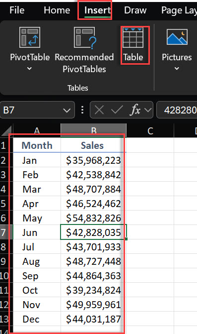
Select your data.
Press Ctrl + T.
Check “My table has headers” if you’ve got column titles.
Hit OK and watch the magic happen.
Real-life scenario: Managing a project task list? Convert it to a table. Now, every time you add a new task, the table will automatically expand, keeping your formatting consistent.
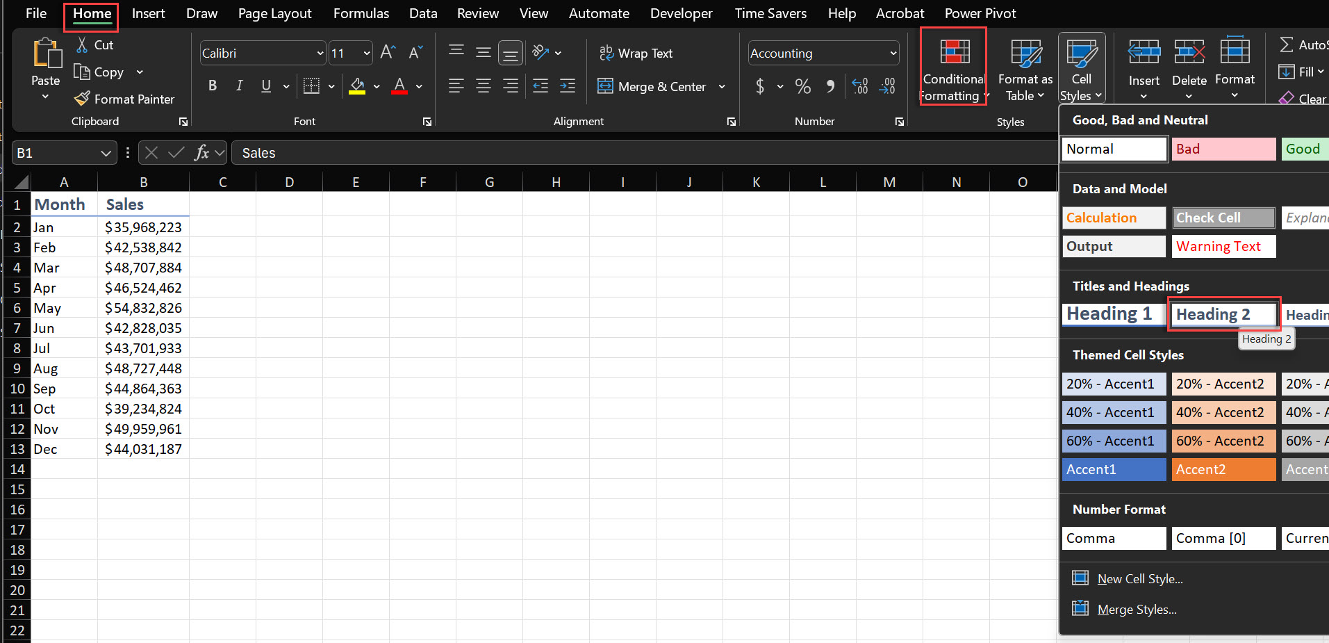
Want to give your spreadsheet a consistent, professional look without spending hours on formatting? Formatting cells is crucial for enhancing the readability and presentation of your data. Cell styles are your secret weapon. While tools like Format Painter can save time, there are instances where you may need to manually format data to ensure it stands out.
How to Wield Them
Select the cells you want to jazz up.
Go to Home > Cell Styles.
Choose from pre-set styles or create your own custom look.
Insider tip: Create a custom style for your company’s branding. Use it for headers across all your reports for a polished, cohesive look.
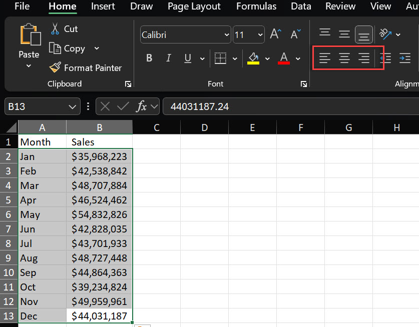
Proper alignment isn’t just about making things look pretty – it’s about making your data easy to read and understand. Horizontal alignment settings can be adjusted for text positioning within cells. When working with protected sheets, the formula bar can be hidden to prevent users from seeing the formulas.
Quick Alignment Hacks
Use the alignment tools in the Home tab (left, center, right).
For vertical alignment, play with top, middle, and bottom options.
Pro move: Center-align your column headers, left-align text data, and right-align numerical data. Your spreadsheet will instantly look more organized and professional.
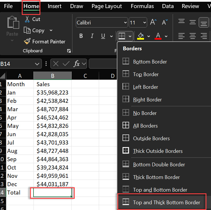
Borders aren’t just for making your spreadsheet look like a fancy table – they’re crucial for organizing and separating data effectively.
Border Basics
Select your cells.
Go to Home > Borders (or use the shortcut Ctrl + Shift + 7 for outlines).
Experiment with different styles and thicknesses.
Expert example: In a budget tracker, use thick borders to separate different expense categories, and lighter borders between individual entries. It’ll make your data easier to navigate at a glance.
To fix data formatting in Excel:
Use the Format Cells dialog:
Select the cells you want to fix.
Right-click and choose “Format Cells” (or use Ctrl + 1).
Select the appropriate category (Number, Date, Text, etc.).
For quick fixes:
Use number format buttons on the Home tab.
Try the “Text to Columns” feature for splitting or combining data.
For dates and times:
Use custom format codes (e.g., “mm/dd/yyyy” or “hh:mm AM/PM”).
To fix text formatted as numbers:
Use the TEXT function: =TEXT(A1,”@”)
Pro Tip: Use Excel’s Flash Fill feature to quickly reformat data based on examples you provide.
To format data in Excel:
Basic formatting:
Use the Home tab for font, alignment, and number formatting.
Apply styles from the “Cell Styles” gallery for quick, consistent formatting.
Conditional Formatting:
Use to highlight cells based on their values.
Go to Home > Conditional Formatting.
Tables:
Convert your data range to a table (Ctrl + T) for automatic formatting and filtering.
Custom Number Formats:
Create custom formats using Format Cells > Number > Custom.
Data Validation:
Set rules for data entry to maintain consistency.
Remember: Consistent formatting across your spreadsheet improves readability and analysis.
To clean and format data in Excel:
Remove duplicates:
Select your data and go to Data > Remove Duplicates.
Fix inconsistencies:
Use PROPER(), UPPER(), or LOWER() functions to standardize text case.
Use TRIM() to remove extra spaces.
Standardize formats:
Use Format Cells to set consistent number, date, and text formats.
Handle missing data:
Use conditional formatting to highlight blanks.
Consider using IF() or IFERROR() to handle empty cells.
Split or combine data:
Use Text to Columns or CONCATENATE() function.
Use Data Validation:
Set rules to prevent incorrect data entry.
Pro Tip: Consider using Power Query (Get & Transform) for more complex data cleaning tasks.
To make data look good in Excel:
Use consistent formatting:
Apply cell styles for titles, headings, and data.
Use a color scheme that’s easy on the eyes.
Align data properly:
Left-align text, right-align numbers, center headings.
Add borders and shading:
Use borders to separate sections.
Apply light shading to header rows.
Use appropriate number formats:
Format currencies, percentages, and dates correctly.
Implement conditional formatting:
Highlight important data or trends.
Adjust column widths and row heights:
Use AutoFit or manually adjust for best appearance.
Use charts and sparklines:
Visualize data trends with appropriate charts.
To create an attractive Excel spreadsheet:
Use a consistent color scheme:
Stick to 2-3 complementary colors.
Use the “Themes” feature for pre-designed color schemes.
Implement a clear hierarchy:
Use larger, bold fonts for main titles.
Use slightly smaller fonts for subheadings.
Utilize white space:
Don’t crowd your data; give it room to breathe.
Add visual elements:
Use charts, graphs, or SmartArt to break up text and numbers.
Format tables professionally:
Use Excel’s built-in table styles for a polished look.
Be consistent with fonts:
Stick to 1-2 professional fonts throughout the spreadsheet.
Use freeze panes:
Keep headers visible as you scroll through large datasets.
Add a title page or dashboard:
Summarize key information attractively.
To improve formatting in Excel:
Learn keyboard shortcuts:
Ctrl + B for bold, Ctrl + I for italic, etc.
Alt + H + O + I for AutoFit column width.
Use styles consistently:
Create and apply custom styles for different elements.
Leverage conditional formatting:
Automatically format cells based on their content.
Master custom number formats:
Create formats tailored to your specific needs.
Use named ranges:
Name frequently used ranges for easier formatting and formula creation.
Implement data validation:
Ensure data consistency with dropdown lists or specific rules.
Learn advanced features:
Explore PivotTables, Power Query, and macros for complex formatting tasks.
Regularly review and update:
Periodically review your spreadsheets to ensure formatting remains relevant and effective.
A cell value in Excel refers to the data or formula contained in a specific cell of a spreadsheet.
You can customize cell borders by selecting the cells, clicking on the “Borders” option in the Home tab, and choosing styles, colors, and thicknesses.
A dialog box in Excel is a pop-up window that allows you to access advanced settings or options, such as formatting cells or managing data.
There you have it – six essential Excel formatting tricks that’ll take your spreadsheets from “meh” to “wow!” With these skills in your toolbox, you’ll be churning out professional-looking reports and data visualizations in no time.

92% of students automate workflows, build CEO-ready dashboards, and streamline collaboration in < 1 hour. Don’t miss out!
🎯Master every Office 365 tool like Excel, Word, PowerPoint, Teams, Outlook and OneNote.
🎯Streamlined approach—no fluff, just rapid skill-building.
🎯Eliminate tedious tasks with intelligent automation.
🎯Transform everyday workflows into strategic power moves.
🎯Boost productivity and impress every boss.
🎯Real-World Projects – directly translate lessons into workplace wins.