This comprehensive guide introduces you to dynamic filtering techniques in Excel that will revolutionize how you handle large datasets. From basic table features to advanced formula-based filtering and interactive slicers, you’ll learn how to create flexible, self-updating filters that save time and enhance data analysis. Perfect for Excel users of all levels looking to streamline their workflow and improve productivity.
by Mihir Kamdar / Last Updated:
After reading this guide, you’ll be equipped with the knowledge to:
Creating dynamic dropdown filters using Data Validation
Advanced filtering techniques with Excel formulas, including the FILTER function and the new dynamic array functions
Implementing interactive Slicers for visual data filtering
Download our step-by-step tutorial file now by clicking on the icon below and follow along to enhance your Excel skills practically and efficiently!
Have you ever found yourself drowning in a sea of Excel data, manually filtering through countless rows just to find the information you need? If so, you’re not alone. Filtering large datasets in Excel can be time-consuming if done manually. But with dynamic filtering techniques, you can save time and boost your efficiency dramatically.
Dynamic filtering in Excel allows you to automatically filter and update your data as it changes. This means less time spent on manual updates and more time for analysis and decision-making. The excel filter function is a powerful tool that helps streamline data management by extracting specific subsets of data based on defined criteria. When utilizing the filter function excel, you can dynamically adjust results as your data changes, making it invaluable for automating processes. The standard excel filter feature enables quick sorting and filtering through dropdown menus, ideal for basic tasks.
If you’re exploring ways to implement filtering, understanding filter excel function ensures that your datasets remain organized and searchable. Learning how to filter in excel is simple—just go to the “Data” tab, click “Filter,” and use the dropdown menus in column headers to display the desired information. The filter excel capability offers flexibility, whether you’re sorting alphabetically or focusing on specific data ranges.
For beginners seeking to learn how to add filter in excel, the process is intuitive, involving a few clicks to apply filters to your datasets. Advanced users might explore the excell simple filter function to handle repetitive tasks more efficiently. Adjusting for changing the filter functunality ensures that your workflows remain effective even with evolving datasets. These techniques combined provide a comprehensive approach to mastering Excel’s filtering tools.
In this guide, we’ll explore various dynamic filtering techniques, from basic table features to advanced formulas and interactive slicers. Whether you’re a beginner or an experienced Excel user, you’ll find valuable tips to streamline your data management process.
The FILTER function in Excel leverages a boolean array to identify rows meeting specified criteria, where TRUE values signify matches. By performing a logical test within the function, users can dynamically extract subsets of data based on customized filter criteria.
This capability is instrumental in filtering data, especially for large datasets, as it ensures precision and automation. Advanced filter functions further enhance flexibility, allowing for the creation of dynamic and self-updating filters that streamline data analysis and improve workflow efficiency.
The FILTER function syntax utilizes dynamic arrays to simplify data management by dynamically adjusting the output size to match the data. These dynamic array formulas allow users to extract matching values from the same column or across multiple columns based on criteria applied to the original data.
This ensures that the results update automatically as the data changes, making it an efficient tool for analyzing large datasets. By combining these features, Excel enhances its capability to filter and organize information effectively.
To filter in Excel, the process is straightforward and can greatly enhance your ability to manage and analyze large datasets. If you’re wondering how do I filter in excel, you simply need to select your data range, go to the “Data” tab, and click on “Filter.” This will activate dropdown arrows in the header cells, allowing you to sort and filter data by specific criteria, such as numbers, text, or dates.
To do multiple filters in excel, you can apply filters on different columns simultaneously. Excel allows users to filter by multiple criteria across different columns, making it easier to focus on specific subsets of data. For example, if you’re working with a sales dataset, you can filter by both region and product type.
The excel filtering functions give you more advanced options. Excel how to use filters involves applying these functions, like using the filter formula excel to extract specific rows of data that meet certain conditions, such as “Sales greater than $500”.
For more complex needs, you might need the function filter excel, such as using the excel formula for filter to automate specific filtering tasks. Another common question is how to filter data in excel based on specific name. You can simply use the text filters or apply a formula to isolate rows with matching names.
If you’re unsure how to excel filter no 0, you can exclude zeros or any unwanted values by using specific criteria or formula-based filtering. Another common requirement is to excel how to filter column from high to low, which you can do by sorting the data in descending order directly from the filter dropdown.
Finally, the filtern excel feature, available in different versions, provides seamless integration for users to quickly filter data in multiple ways. With these methods, you can efficiently manage data and enhance your workflow.
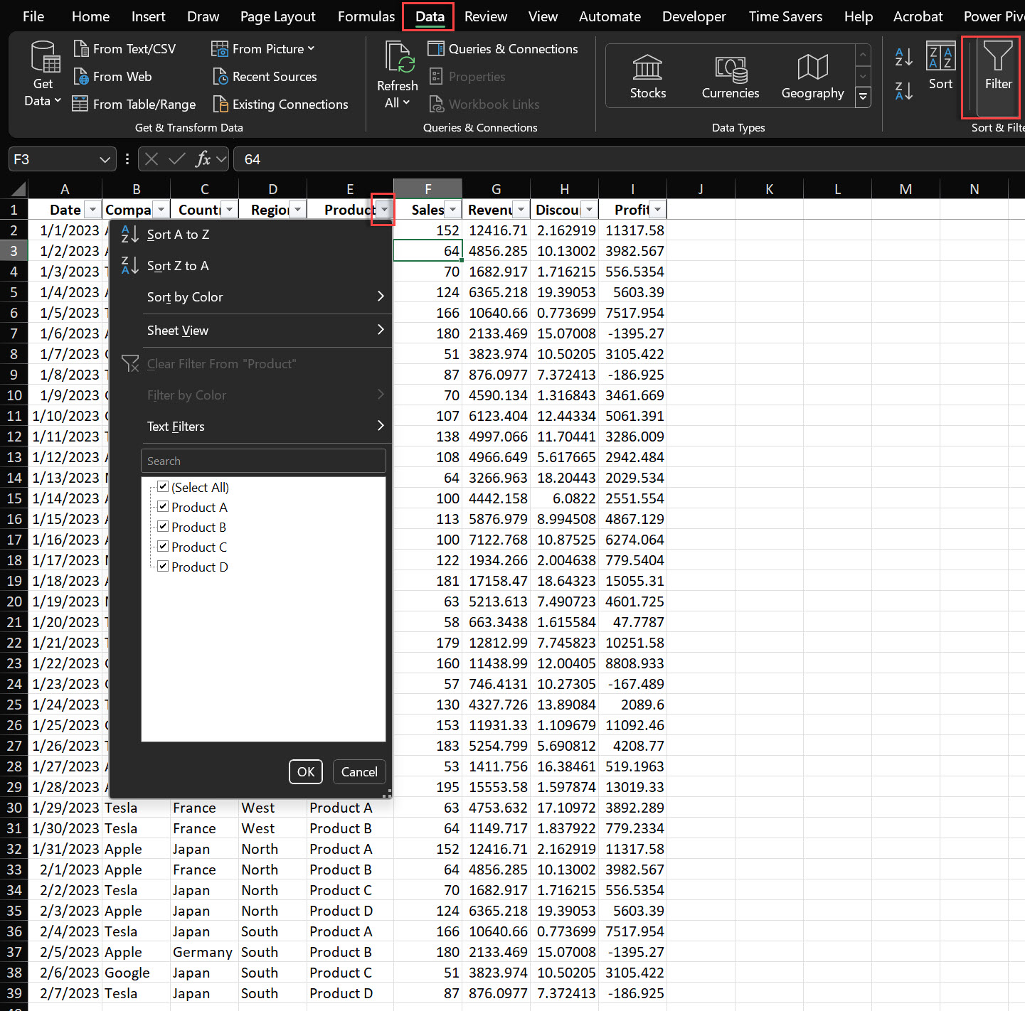
Before we dive into dynamic techniques, let’s quickly review Excel’s basic filtering options. These are found under the Home tab in the Sort & Filter group.
To apply a basic filter:
Select any cell within your data range.
Click on the Filter button in the Sort & Filter group.
Click the dropdown arrow in the header cell of the column you want to filter.
Select the values you want to display or use the search box to find specific items.
For example, if you have a sales dataset, you might filter by month to show only January sales, or by region to focus on a specific market area or focus on specific product.
While useful, these basic filters have limitations. They don’t automatically update as your data changes, and they can be cumbersome for large datasets. This is where dynamic filtering comes in.

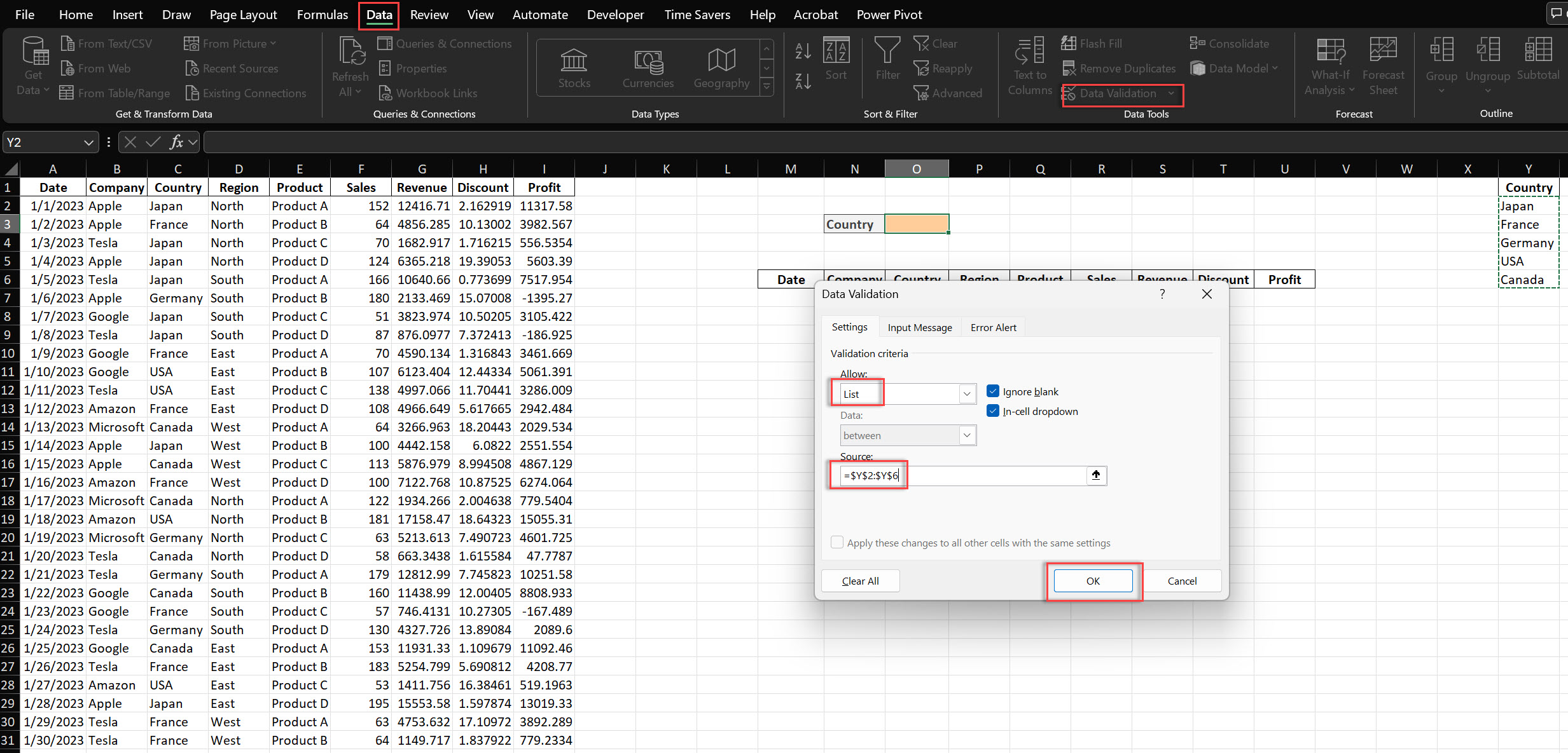
Data Validation allows you to create custom dropdown lists that can be used to filter your data dynamically.
Excel Tables allow you to filter all the columns efficiently, ensuring that your data remains manageable and organized.
Here’s how to set it up:
Create a list of your filter categories (e.g., Country) in a separate column.
Select the cell O3 where you want your dropdown to appear.
Go to Data > Data Validation.
In the Settings tab, set Allow to “List”.
For Source, select your list of countries from Y2:Y6.

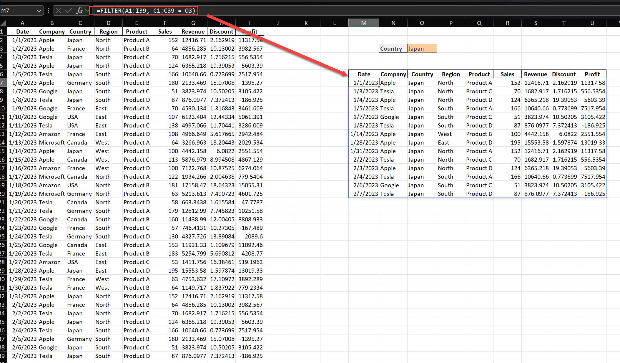
To connect this dropdown to your data:
Use a formula like =FILTER(A1:I39, C1:C39 = O3), where O3 is your dropdown cell. Type this formula in cell M7.
This formula will filter your data based on the selected country in the dropdown.
This technique is particularly useful for creating interactive reports where users can select different views of the data without needing to understand Excel’s built-in filter functionality.

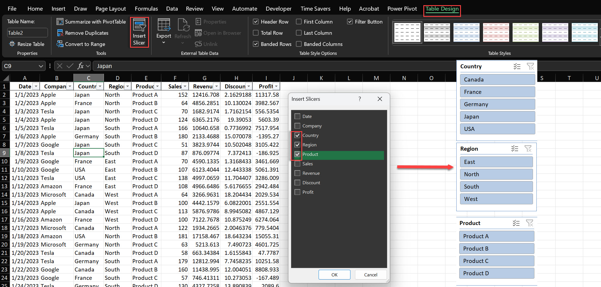
Slicers provide a visual, interactive way to filter your data. They’re especially useful for dashboards or reports where you want users to be able to easily explore the data.
For case-sensitive filtering, you can use the EXACT function within your filter formula. This ensures that only data matching the exact case of your criteria is included.
To add a slicer:
Click anywhere in your Excel Table.
Go to Table Tools > Insert Slicer.
Select the column(s) you want to create slicers for.
Slicers will appear as buttons that users can click to filter the data. You can add multiple slicers to filter by different criteria simultaneously.
For example, in a sales dashboard, you might have slicers for Product, Region and Country. Users can then click on these slicers to instantly filter the data and see different views, such as “Product 1″ sales in the North region of Japan.

Using Excel filters is straightforward:
Select the range of data you want to filter.
Go to the “Home” tab and click on “Sort & Filter” > “Filter”.
Click the arrow in the column header you want to filter.
Choose the criteria you want to filter by (e.g., specific values, text contains, etc.).
Your data will now be filtered based on your selection.
Pro Tip: Use keyboard shortcut Ctrl + Shift + L to quickly toggle filters on and off.
To add a drop-down filter:
Select the cell where you want the drop-down.
Go to “Data” tab > “Data Validation”.
In the “Allow” box, select “List”.
In the “Source” box, enter your list items separated by commas or refer to a range of cells.
Click “OK”.
Now you have a drop-down list that can be used to filter your data.
To add a filter button:
Select the range of data you want to filter.
Go to the “Home” tab.
In the “Editing” group, click on “Sort & Filter”.
Select “Filter”.
Filter buttons will appear in the header row of your selected range.
Shortcut: Use Ctrl + Shift + L to quickly add or remove filter buttons.
The FILTER function in Excel allows you to filter and sort data in one step:
Syntax: =FILTER(array, include, [if_empty])
Example: =FILTER(A1:B10, A1:A10>5, “No results”) This filters rows where column A is greater than 5.
To sort, combine with SORT function: =SORT(FILTER(A1:B10, A1:A10>5), 2, 1) This sorts the filtered results by column B in ascending order.
To use Advanced Filter:
Set up a criteria range above your data (include column headers).
Select your data range.
Go to “Data” tab > “Advanced” in the Sort & Filter group.
In the Advanced Filter dialog:
Choose to filter the list in-place or copy to another location.
Specify the List range and Criteria range.
Click “OK”.
Advanced Filter allows for more complex criteria than regular filters, including using formulas as criteria.
The FILTER function in Excel is a dynamic array formula that extracts matching data from a range based on specific criteria. It updates automatically when data changes.
Dynamic filtering in Excel is a game-changer for anyone working with large datasets. By using techniques like Excel Tables, Data Validation dropdowns, advanced formulas, and Slicers, you can create flexible, interactive reports and dashboards that update automatically as your data changes. By mastering how to filter in Excel, you can efficiently manage and analyze filtered data, making your workflow more productive.

92% of students automate workflows, build CEO-ready dashboards, and streamline collaboration in < 1 hour. Don’t miss out!
🎯Master every Office 365 tool like Excel, Word, PowerPoint, Teams, Outlook and OneNote.
🎯Streamlined approach—no fluff, just rapid skill-building.
🎯Eliminate tedious tasks with intelligent automation.
🎯Transform everyday workflows into strategic power moves.
🎯Boost productivity and impress every boss.
🎯Real-World Projects – directly translate lessons into workplace wins.