Learn how to master Excel’s XLOOKUP and 2-way XLOOKUP functions. Perfect for modern data analysis, this comprehensive guide includes practical examples and expert tips. Updated for Excel 2024.
by Mihir Kamdar / Last Updated:
After reading this guide, you’ll be equipped with the knowledge to:
Download our step-by-step tutorial file now by clicking on the icon below and follow along to enhance your Excel skills practically and efficiently!
Are you missing VLOOKUP already? Don’t worry! XLOOKUP is here to make your Excel life easier. Let’s learn how this powerful function can transform your lookup data experience. The lookup array refers to the first column (e.g., column A) where Excel searches for the lookup value. Moreover, the return array corresponds to the column number (e.g., column B) containing the values to be retrieved. The equivalent VLOOKUP formula for =XLOOKUP(“Gabriel Parr”, A:A, B:B, “Not Found”) is =VLOOKUP(“Gabriel Parr”, A:B, 2, FALSE).
If we do a XLOOKUP vs VLOOKUP comparison, excel XLOOKUP is more versatile than VLOOKUP, allowing searches in any direction, eliminating the need for sorted data, and handling errors more efficiently with customizable outputs. There is a noticeable difference between vlookup vs xlookup comparison.
In an exact match XLOOKUP, the lookup value is the specific value you want to find, such as “Gabriel Parr.” The lookup array is the range or lookup column where Excel searches for the lookup value, like column A containing names. For example, the formula =XLOOKUP(“Gabriel Parr”, A:A, B:B, “Not Found”) looks for “Gabriel Parr” in column A and returns the corresponding value from column B. If no match is found, it returns “Not Found.” By default, XLOOKUP performs an exact match, making it ideal for precise data retrieval.
XLOOKUP wildcard does not work with number values unless additional formatting adjustments are made. Google Sheets XLOOKUP alternatives allow users to mimic similar functionality for data lookups. XLOOKUP match mode includes options for exact, approximate, and wildcard matches for greater flexibility. The difference between VLOOKUP and XLOOKUP lies in its flexibility, bidirectional lookups, and error handling. How to use XLOOKUP in Excel involves understanding its syntax and applying it for efficient lookups. How to use XLOOKUP function in Excel shows its ability to replace traditional lookup methods with ease.
The XLOOKUP function is a powerful and flexible tool in Excel that allows you to search for a value in a range or array and return a corresponding value from the same row. It’s a modern replacement for the VLOOKUP function, offering several advantages such as faster performance and a more flexible syntax. One of the standout features of the XLOOKUP function is its support for wildcards and binary search, making it incredibly versatile. Whether you need to perform exact matches, approximate matches, or wildcard matches, XLOOKUP has got you covered.
The XLOOKUP function has the following syntax: =XLOOKUP(lookup_value, lookup_array, return_array, [if_not_found], [match_mode], [search_mode]). Here’s a breakdown of the arguments:
Optional arguments include:
The Power of XLOOKUP
Think of XLOOKUP Excel as the Swiss Army knife of lookup functions. Unlike its predecessors (VLOOKUP and HLOOKUP), XLOOKUP can:
Simple Yet Powerful Syntax
Basic XLOOKUP Formula:
=XLOOKUP(lookup_value, lookup_array, return_array, [if_not_found])
Let’s break it down:
XLOOKUP offers more advanced capabilities compared to traditional match functions like VLOOKUP and INDEX-MATCH.
Wildcard matches allow for flexible data searching. Additionally, partial matches can help identify values that may be misspelled or entered incorrectly, enhancing the search process within large datasets.
=XLOOKUP(F2, C:C, A:A, “Not Found”)
This means:
The ‘if_not_found’ argument allows you to specify what to display if the search value is not found. You can also adjust the search criteria to tailor your queries, making it easier to efficiently search through data sets. This flexibility allows users to customize their search parameters when using functions like XLOOKUP.

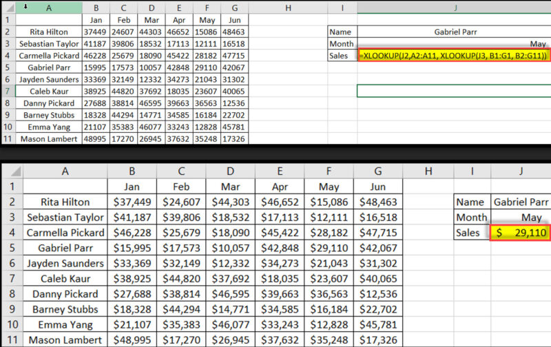
Imagine finding a value using both row and column criteria – like looking up a price that matches both a product AND a size.
The Formula:
=XLOOKUP(J2, A2:A11, XLOOKUP(J3, B1:G1, B2:G11))
Real Example: Finding Gabriel’s May sales:
Breaking It Down:

XLOOKUP is a versatile lookup function in Excel that can search for a value in a range and return a corresponding value from another range.
XLOOKUP is more flexible – it can look left or right, doesn’t require sorting, and can return multiple values. It’s generally considered an improvement over VLOOKUP.
=XLOOKUP(lookup_value, lookup_array, return_array, [if_not_found], [match_mode], [search_mode])
By default, it returns #N/A. You can specify a custom value using the [if_not_found] argument.
Yes, by setting the match_mode argument to -1 or 1.
XLOOKUP isn’t just another Excel function – it’s your new best friend for finding data quickly and accurately. Start using it today, and you’ll wonder how you ever lived without it!
XLOOKUP multiple criteria enable users to perform advanced lookups with enhanced accuracy. XLOOKUP returning values simplifies the process of extracting data efficiently. The XLOOKUP formula provides a user-friendly structure for performing lookups in Excel.
Furthermore, the XLOOKUP Google Sheets functionality can be replicated using alternative methods for similar results. Excel not showing XLOOKUP function often occurs due to outdated versions or unsupported features.
My Office 365 is not giving me XLOOKUP in Excel due to potential subscription or update issues. An XLOOKUP example illustrates how it simplifies data retrieval tasks in various scenarios. XLOOKUP to add multiple values combines lookup capabilities with aggregation functions for dynamic results.
Moreover, the XLOOKUP vs INDEX MATCH highlights the advanced capabilities and simplicity of XLOOKUP over traditional methods.

92% of students automate workflows, build CEO-ready dashboards, and streamline collaboration in < 1 hour. Don’t miss out!
🎯Master every Office 365 tool like Excel, Word, PowerPoint, Teams, Outlook and OneNote.
🎯Streamlined approach—no fluff, just rapid skill-building.
🎯Eliminate tedious tasks with intelligent automation.
🎯Transform everyday workflows into strategic power moves.
🎯Boost productivity and impress every boss.
🎯Real-World Projects – directly translate lessons into workplace wins.