Power Query: A Comprehensive Guide to Extract, Transform, and Load (ETL) in Excel

Power Query is a powerful tool in Excel that simplifies the process of extracting, transforming, and loading (ETL) data. Whether you’re dealing with large datasets or performing complex analysis, Power Query allows you to clean, organize, and automate your data effortlessly, saving you time and boosting your productivity.

Dynamic Date Example

by Mihir Kamdar / Last Updated:

C968 Power Query Course 2

What You'll Learn

This guide takes you through each feature of Power Query with practical applications and detailed explanations of every transformation. Here’s what you’ll learn:

  • Learn the basics of the main layout, ribbon, navigation pane, and other pieces of the puzzle for managing data.
  • Guidance on step by step on how to import data from text files, Excel workbooks and Access databases.
  • Basic cleaning techniques such as removing duplicates, replacing null values, merging columns, etc.
  • Learn to use more advanced functions such as unpivoting, pivoting, conditional columns, custom columns, and column splitting.
  • See when and how to use append vs. merge functions to merge data from multiple sources.
  • Methods for exporting and reloading transformed data into Excel, for additional analysis and presentation.

Download File

Download our step-by-step tutorial file now by clicking on the icon  download icon 1  below and follow along to enhance your Excel skills practically and efficiently!

Introduction

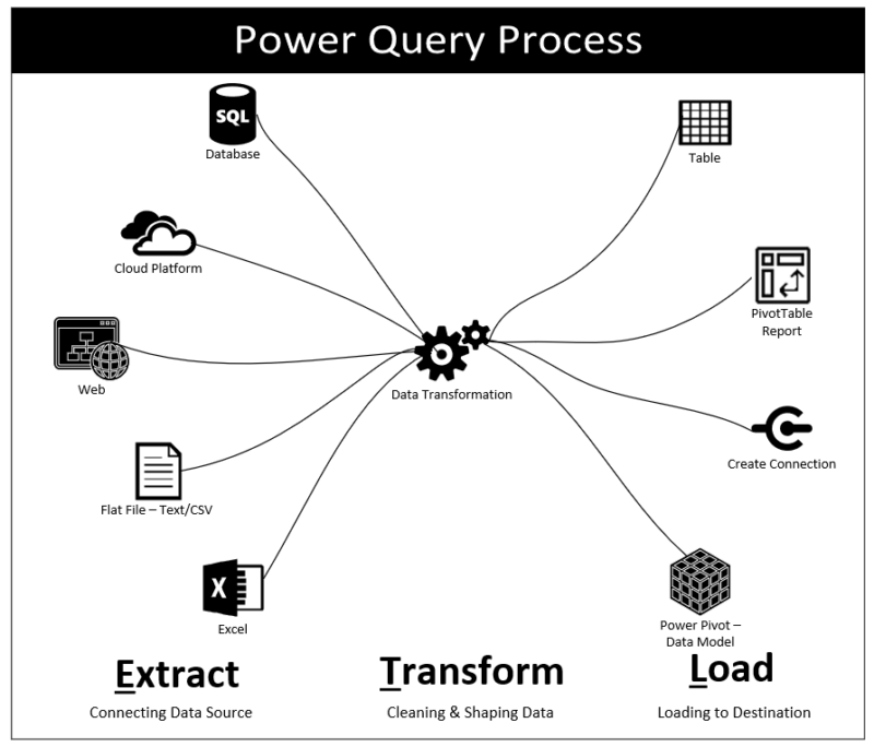
More and more, we live in a data-driven world and dealing with large quantities of data is what organizations and professionals find important. Microsoft Excel has an amazing tool for simple ETL (extract, transform, load) processes referred to as Power Query, which simplifies this process very well. If you are looking for a complete guide to learn about Power Query’s most important tools and functions, which will make you the master of doing the most complex transformations in the easiest and most efficient way this is the place to gather all your information!

power_query_process

1. Power Query User Interface

The Power Query User Interface (UI) makes data transformation easy with a complete set of tools accessible through a simple UI. To efficiently manage, clean and transform data, you need to understand the layout and the function of each component. Here’s a breakdown of the key components in the Power Query UI:

  1. Ribbon: Positioned at the top of the Power Query window, the ribbon includes several tabs—HomeTransformAdd Column, and View—each packed with essential commands. The Home tab offers common transformations like removing duplicates, renaming columns, and applying filters.
  2. Query Navigation Pane: Located on the left side, this pane lists all the queries within the workbook. Each query represents a different data source or transformation sequence, which users can toggle between.
  3. Formula Bar: The formula bar, at the top of the editor, displays the M language code behind each transformation. Power Query uses M, a functional language designed specifically for data transformations.
  4. Preview Pane: The Preview Pane shows a sample of the data currently loaded into the query. As users apply transformations, this pane updates in real-time, reflecting each change.
  5. Properties and Query Settings: Found on the right, this window displays the properties of the current query, such as its name and load destination. Below, the Applied Steps list records each transformation applied to the data, with options to edit, delete, or reorder steps.

Power Query editor

Excel: Free Masterclass​
Supercharge Your Skills For Free

2. Import Data – Text File

Text files are one of the simplest data sources to import, and Power Query supports a range of options for integrating them into your workflow. Below is a step-by-step guide to creating queries from text files, specifically for Order Priority and Sales Channel.

Importing the First Text File (Order Priority)
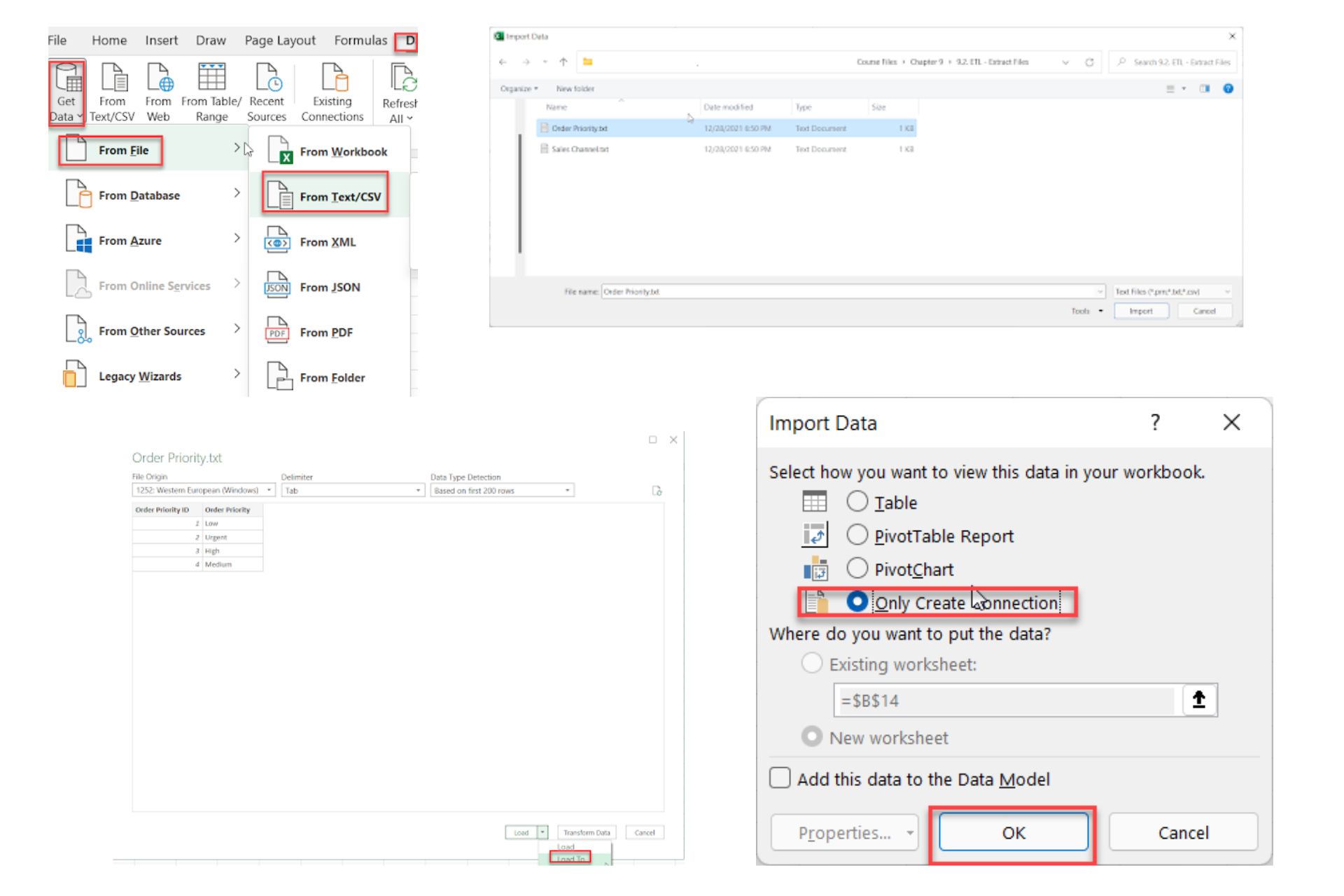
  1. Access the Import Tool: Open Excel and navigate to Data > Get Data > From File > From Text/CSV. This will prompt you to select the text file you wish to import.
  2. Select the File: Browse your system, select Order Priority.txt, and click Import. A preview of the data will appear, showing the structure and allowing you to confirm it’s correct.
  3. Load Options: Click on Load To, which will bring up different loading options. To keep the data connected without displaying it in the workbook, select Only Create Connection.
  4. Confirm and Create Connection: Click OK to finalize the connection. This setup will dynamically update whenever the text file’s data changes, maintaining a live link in your query list.
Import Data from Text File

Importing the Second Text File (Sales Channel)

  1. Open Import Tool: Once again, go to Data > Get Data > From File > From Text/CSV.
  2. Select Sales Channel File: This time, select Sales Channel.txt, then click Import to preview the file.
  3. Load to Connection Only: As with the first file, click Load To and select Only Create Connection. This choice allows you to work with the data in Power Query without loading it directly into Excel until needed.
  4. Confirm Connection: Click OK to complete the process. Now, both text files are set up as live connections within the query navigation pane, ready for transformations or integration with other data sources.

Import Data Text File

Excel: Free Masterclass​
Supercharge Your Skills For Free

3. Import Data – Excel File

Excel workbooks are a common source for data storage, and Power Query provides a straightforward method for importing data directly from these files. By connecting to Excel files, you can dynamically update and integrate data without manually copying or opening each file. Below is a step-by-step guide on importing data from an Excel workbook into Power Query, specifically for the Order Sales Transaction.xlsx file.

  1. Access the Import Tool: Open Excel, go to Data > Get Data > From File > From Workbook. This opens a file browser where you can locate the Excel file you want to import.
  2. Select the Excel File: Browse for and select Order Sales Transaction.xlsx, then click Import. Power Query will display a list of available worksheets and tables within the workbook.
  3. Choose the Data Sheet: In the navigator window, select the specific sheet or table you wish to import, in this case, dim_SalesTransaction. A preview of the data will appear on the right side, allowing you to confirm that it’s the correct dataset.
  4. Load Options: After selecting the correct sheet, click on Load To. Choose Only Create Connection to set up a live link to the data without loading it directly into your workbook. This option is helpful for managing data that might be frequently updated, as it allows Power Query to refresh the connection whenever changes are made to the source file.
  5. Confirm Connection: Press OK to finalize the connection. The query will appear in the Power Query navigation pane, ready for any transformations you may need.

Untitled design 48

Excel: Free Masterclass​
Supercharge Your Skills For Free

4. Import Data – Access Database

Microsoft Access databases are often used for managing relational data, and Power Query allows for easy integration of these datasets into Excel. Here’s how to import data from an Access database, specifically from the Order Other Data.accdb file, while setting up a dynamic connection.

  1. Access the Import Tool: In Excel, go to Data > Get Data > From File > From Workbook. This opens a file browser where you can locate and select the Access database file.
  2. Select the Database File: Find Order Other Data.accdb and click Import. Power Query will open a navigator displaying available tables and queries within the database.
  3. Select Multiple Tables: In the navigator, select multiple tables by clicking on each required table (e.g., fct_Customer, fct_Date, fct_ItemType, fct_Location). After confirming the selections, click Load To.
  4. Load as Connection Only: Choose Only Create Connection to set up a live link without loading the data directly into Excel. Press OK to finalize.

5. Import Data Access Database

Excel: Free Masterclass​
Supercharge Your Skills For Free

5. Renaming Query

Renaming queries in Power Query improves organization and readability, especially when working with multiple data sources. By assigning clear, descriptive names to each query, you can easily identify and manage them throughout your analysis.

  1. Open the Queries Pane: In the Power Query editor, locate the Queries pane on the left side, which lists all active queries.
  2. Rename Each Query: To rename, right-click on each query (e.g., fct_SalesTransaction, dim_OrderPriority, dim_SalesChannel, dim_Customer, dim_Date, dim_ItemType, dim_Location). Select Rename or use the Properties Window on the right side to change the name.
  3. Confirm Renaming: After renaming, each query will display its new name in the Queries pane, creating a structured and organized view that’s easier to navigate.

6. Renaming Query

Excel: Free Masterclass​
Supercharge Your Skills For Free

6. Remove Duplicates

Removing duplicate rows is essential for data accuracy, particularly when working with large datasets. In Power Query, this function can quickly identify and eliminate repeated entries to ensure each row in the dataset is unique.

  1. Select the Query: In the Power Query editor, open the fct_SalesTransaction query where duplicate rows need to be removed.
  2. Select All Rows: In the Preview Pane, click anywhere within the data and press Ctrl + A to highlight all rows.
  3. Remove Duplicates: Right-click on any highlighted column and select Remove Duplicates from the context menu. Power Query will automatically identify and remove any duplicate entries.

image25

Excel: Free Masterclass​
Supercharge Your Skills For Free

7. Replace Null Values

Replacing blank or null values is essential to maintain data consistency, especially when performing calculations. In Power Query, you can replace all null values with a specific number, such as “0,” in designated columns to avoid errors in analysis.

  1. Open the Query: In the Power Query editor, open the fct_SalesTransaction query.
  2. Select Columns: Select the last three columns where blank values are displayed as null.
  3. Replace Null Values: Right-click on any of the selected columns and choose Replace Values. In the Value To Find box, type null, and in the Replace With box, enter 0. Press OK to apply.

Alternatively, you can go to Home > Transform > Replace Values to enter the same details.

Replace Null Values

Excel: Free Masterclass​
Supercharge Your Skills For Free

8. Replace Blank Values

Replacing blank strings in data is crucial for maintaining clarity, especially when fields are expected to contain text. In Power Query, blank strings within text fields can be filled with a placeholder, such as “Not Available,” ensuring that missing values are clearly identified.

  1. Open the Query: In the Power Query editor, select the dim_Customer query.
  2. Select Columns with Blank Strings: Highlight the last three columns where blank strings (displayed as ” “) appear.
  3. Replace Blank Strings: Right-click on any of the selected columns and choose Replace Values. In the Value To Find field, type a single space (” “), and in the Replace With field, enter “Not Available”. Press OK to apply the replacement.

Alternatively, navigate to Home > Transform > Replace Values and enter the same values.
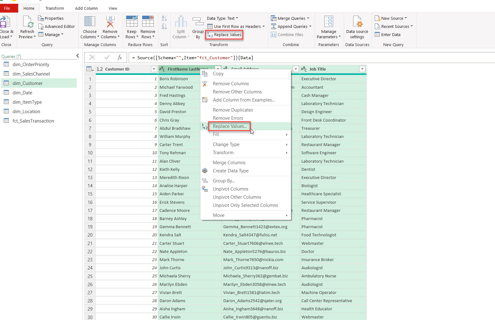
image2 image3

Excel: Free Masterclass​
Supercharge Your Skills For Free

9. Change Text Case

Standardizing the text case in data columns helps maintain consistency, especially for fields like email addresses, which are typically stored in lowercase. In Power Query, changing text to lowercase is straightforward and ensures uniformity across records.

  1. Open the Query: In the Power Query editor, go to the dim_Customer query.
  2. Select the Email Address Column: Click on the Email Address column to highlight it.
  3. Convert to Lowercase: Right-click on the column and select Transform > Lowercase. Alternatively, you can go to Transform > Text Column > Format > Lowercase.

Power Query will immediately apply the transformation, converting all text in the Email Address column to lowercase. This standardization is particularly useful when working with data where case sensitivity may affect analysis or matching processes.

image4

Excel: Free Masterclass​
Supercharge Your Skills For Free

10. Merge Columns

Merging columns in Power Query can create more concise data by combining related information into a single field. In this example, the Region and Country columns in the dim_Location query will be merged to form a unified Region-Country field.
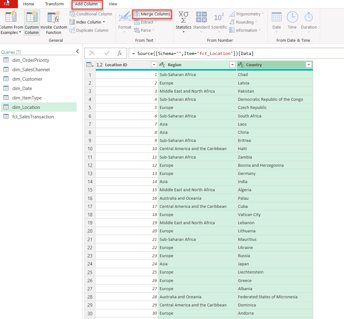
  1. Open the Query: In the Power Query editor, select the dim_Location query.
  2. Select Columns to Merge: Highlight the Region and Country columns.
  3. Merge Columns: Go to Add Column > Merge Columns. In the dialog box, select a separator, such as a hyphen (), to separate the Region and Country values. Enter the new column name as Region-Country.
  4. Apply Changes: Click OK to finalize. Power Query will combine the Region and Country data into the new Region-Country column.

image5 image6

Excel: Free Masterclass​
Supercharge Your Skills For Free

11. Trim & Clean

Removing extra spaces and special characters ensures that data fields are standardized, which is particularly important for text-based columns like Country. In Power Query, you can use the Trim and Clean functions to tidy up text fields, improving data consistency and accuracy.

  1. Open the Query: In the Power Query editor, select the dim_Location query.
  2. Trim Extra Spaces: Click on the Country column to highlight it. Right-click on the column and select Transform > Trim. This function removes any leading or trailing spaces within each entry. Alternatively, you can go to Transform > Text Column > Format > Trim.
  3. Remove Special Characters: With the Country column still selected, right-click and choose Transform > Clean to eliminate any special characters. This ensures that only standard alphanumeric text remains in the column.

Applying Trim and Clean creates a consistent, space-free format for the Country data, which is essential for accurate data processing and analysis.
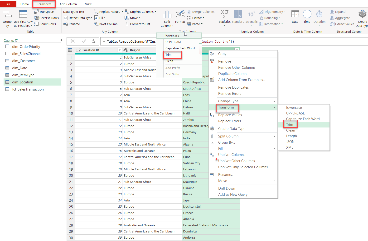
image8 image9

Excel: Free Masterclass​
Supercharge Your Skills For Free

12. Split Column

Power Query allows you to split a single column into multiple columns based on a delimiter, making it easy to separate data fields like full names into first and last names. In this example, we’ll split the First & Last Name column in the dim_Customer query.

  1. Open the Query: In the Power Query editor, select the dim_Customer query.
  2. Select the Column to Split: Click on the First & Last Name column to highlight it.
  3. Split by Delimiter: Go to Transform > Text to Column > Split Column and select By Delimiter. In the dialog box, specify the delimiter (such as a space or comma) that separates the first and last names. Press OK to apply the split.

Power Query will now divide the First & Last Name column into two separate columns, providing distinct fields for each name. This operation is especially helpful for organizing data where individual elements need to be analyzed separately.
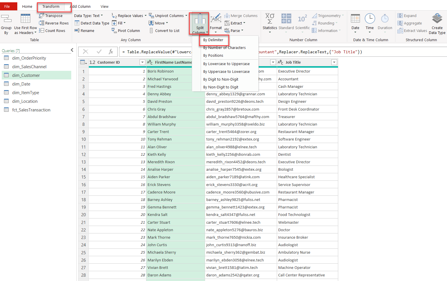
image40 image41

Excel: Free Masterclass​
Supercharge Your Skills For Free

13. Extract Data

The Extract Data function in Power Query enables users to pull specific information from a column, allowing for detailed data extraction, such as isolating certain characters or text patterns. This functionality is particularly useful when you need to retrieve particular portions of data from a single field.

  1. Open the Query: In the Power Query editor, select the query where you want to extract specific data from a column.
  2. Select the Column to Extract Data From: Click on the relevant column containing the data you want to extract.
  3. Apply Extraction Method: Go to Transform > Text Column > Extract and choose the appropriate extraction option:
    • Text Before Delimiter: Extracts text before a specified character or pattern.
    • Text After Delimiter: Extracts text after a specified character or pattern.
    • Text Between Delimiters: Extracts text located between two specified delimiters.
  4. Confirm Extraction: Enter the delimiter(s) as prompted, then press OK. Power Query will display the extracted data in a new column.

Using Extract Data refines the dataset by isolating specific elements, making it easier to analyze particular segments of information without manual filtering.
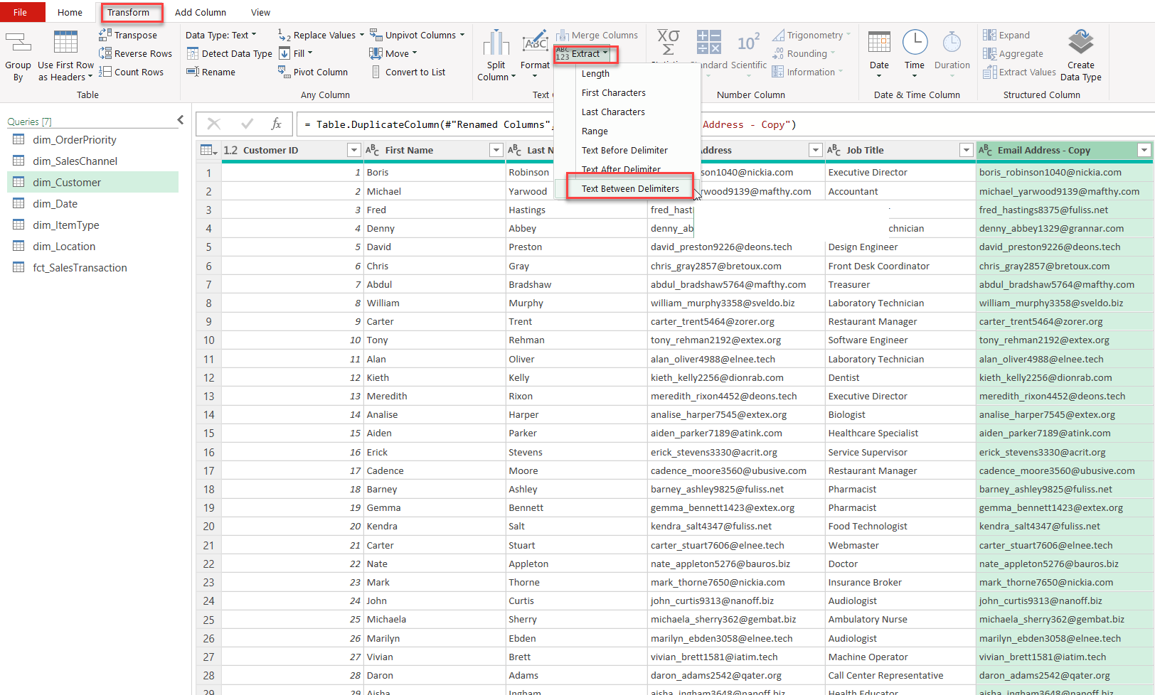
image44 image45

Excel: Free Masterclass​
Supercharge Your Skills For Free

14. Unpivot Column

The Unpivot Columns feature in Power Query is useful for reshaping data by converting selected columns into attribute-value pairs, making analysis and visualization easier. In this case, the columns Units Sold, Unit Price, and Unit Cost in the fact_SalesTransaction query will be unpivoted.

  1. Select Columns to Unpivot: In the Power Query editor, go to the fact_SalesTransaction query. Select the Units Sold, Unit Price, and Unit Cost columns.
  2. Apply Unpivot Columns: Right-click on any of the selected columns and choose Unpivot Columns. Alternatively, you can go to Transform > Any Column > Unpivot Columns.

This action creates two new columns: one for the original column names (Attribute) and another for the corresponding values (Value). The unpivoted data structure is ideal for scenarios requiring summarized data in a single column, enhancing compatibility with pivot tables and charts for deeper analysis.
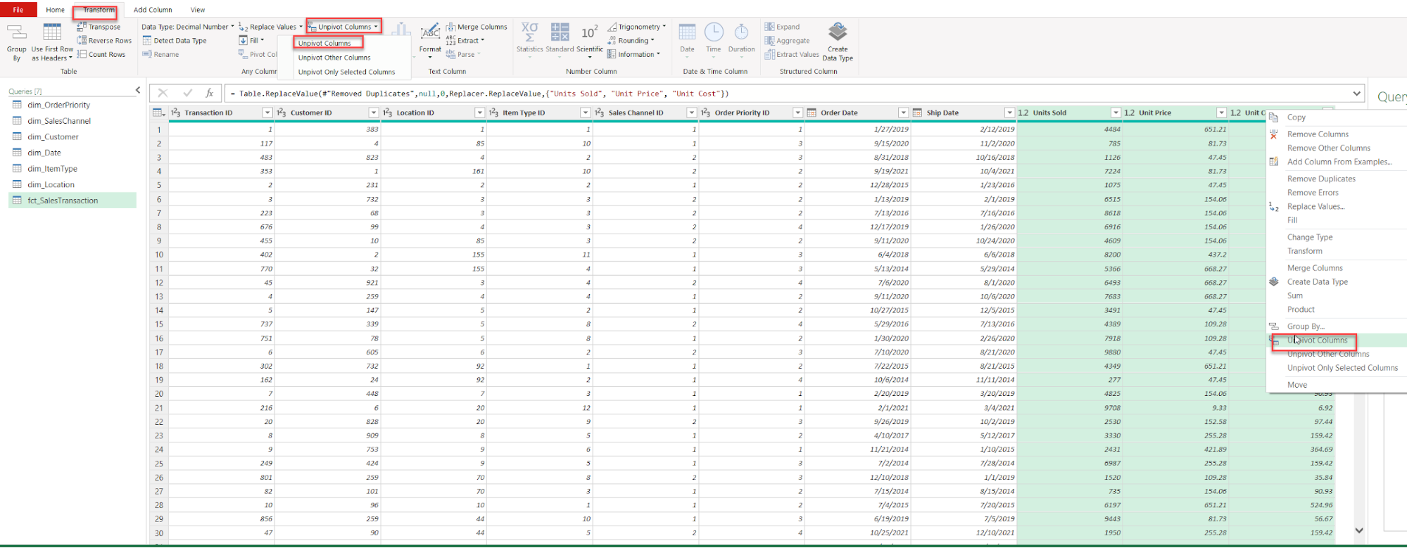
image47 image48

Excel: Free Masterclass​
Supercharge Your Skills For Free

15. Pivot Column

The Pivot Column feature in Power Query allows you to reorganize data by turning attribute-value pairs into distinct columns. This is particularly useful for reversing an unpivoted dataset to restore it to its original column layout. Here, we’ll pivot the fact_SalesTransaction query to recreate the Units Sold, Unit Price, and Unit Cost columns.

  1. Select Columns for Pivoting: In the Power Query editor, select the two columns containing the attribute and value pairs created from the unpivoting process (e.g., Attribute and Value).
  2. Apply Pivot Column: Go to Transform > Any Column > Pivot Column. This option will restore Units Sold, Unit Price, and Unit Cost to individual columns as they were originally.
  3. Confirm and Apply: Press OK to finalize the pivot. The data will now be displayed in separate columns, making it easier to view and analyze each measure individually.

Pivoting columns organizes data neatly, enhancing readability and compatibility with Excel’s native functions.
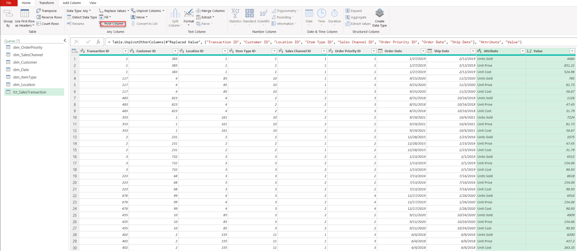
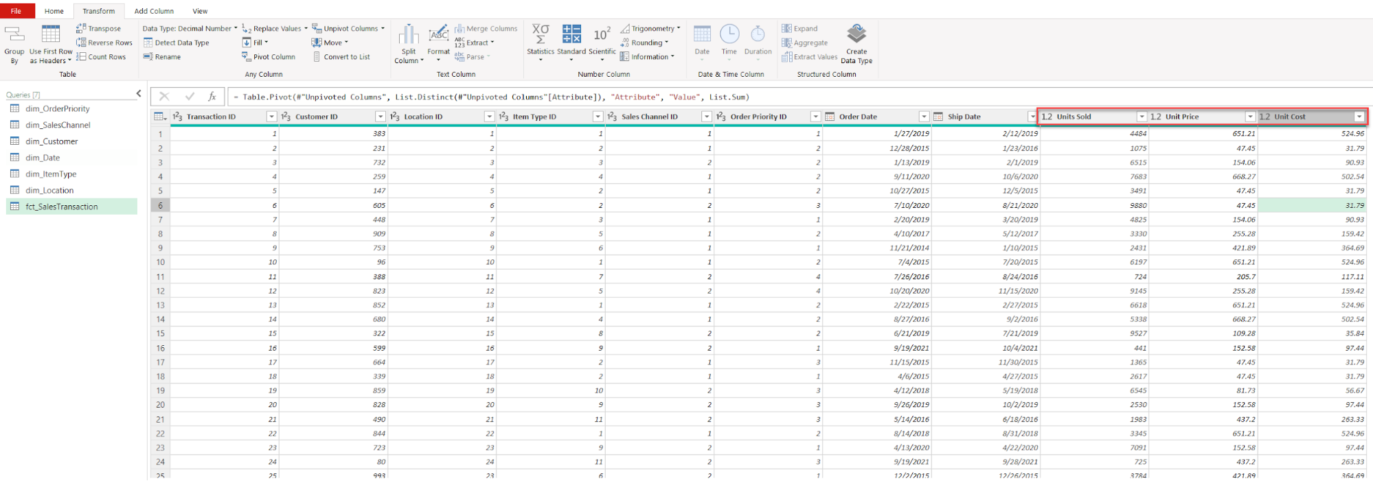
image38 image30 image29

Excel: Free Masterclass​
Supercharge Your Skills For Free

16. Conditional Column

The Conditional Column feature in Power Query allows you to create new columns based on specific conditions within your data. Here, we’ll set up a conditional check in the dim_Location query to identify rows where the word “Africa” appears in the Region column, labeling them accordingly.

  1. Open the Query and Access Conditional Column: In the Power Query editor, open the dim_Location query. Go to Add Column > General > Conditional Column.
  2. Set Condition and Labels: In the conditional column setup, specify the condition: if Region contains the word “Africa,” the new column should display “Africa”; otherwise, it should display “Non-Africa.”
  3. Apply the Conditional Column: After entering the condition and labels, press OK to apply. Power Query will generate a new column with labels based on whether “Africa” is found in the Region field.

This conditional labeling makes it easier to categorize and filter data based on geographic regions.

image31image32image33

Excel: Free Masterclass​
Supercharge Your Skills For Free

17. Multiply Two Columns

In Power Query, multiplying columns allows you to create a new column that represents the product of two existing numerical columns, which is particularly useful for calculating metrics such as total revenue or cost. Here’s how to set up a multiplication in Power Query.

  1. Select Columns to Multiply: In the Power Query editor, highlight the two numerical columns you wish to multiply (for example, Quantity and Unit Price).
  2. Apply Multiplication: Go to Add Column > From Number > Standard > Multiply. Power Query will automatically create a new column containing the product of the selected columns.
  3. Rename the Column (Optional): After multiplication, rename the resulting column to something descriptive, like Total Revenue or Total Cost, to clarify its purpose in your dataset.

image35

Excel: Free Masterclass​
Supercharge Your Skills For Free

18. Custom Column

Creating a Custom Column in Power Query allows for complex calculations and transformations based on specific needs. Here’s a guide to setting up a custom calculation in the fct_SalesTransaction query.
  1. Create a Duplicate Query: Start by duplicating the fct_SalesTransaction query. This provides a separate copy to work with, preserving the original data for reference.
  2. Multiply Columns for Revenue Calculation: Select two relevant columns (e.g., Quantity and Unit Price), and go to Add Column > From Number > Standard > Multiply to create a new Revenue column. Change the data type of this new column to Currency – $ for financial consistency.
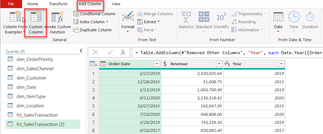
  3. Add Year from Order Date: Select the Order Date column and go to Add Column > From Date & Time > Date > Year to create a new column with only the year value from each order date.
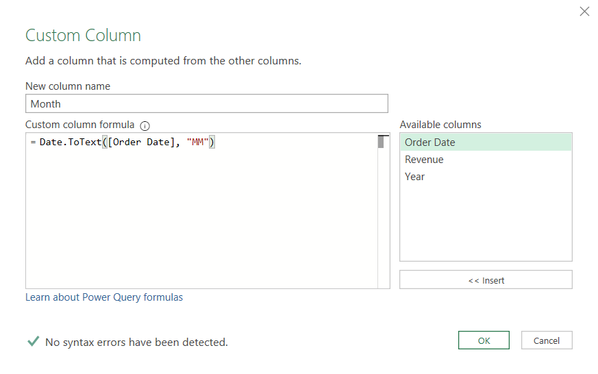
  4. Custom Formula in a New Column: With Order Date selected, navigate to Add Column > General > Custom Column to set up a custom formula, adjusting values or conditions as needed.

image28 image63 image64

Excel: Free Masterclass​
Supercharge Your Skills For Free

19. Group By

The Group By function in Power Query allows you to aggregate data based on specific columns, summarizing large datasets into meaningful insights. In this example, we’ll group data in the duplicated fct_SalesTransaction query by Year and calculate total Revenue for each period.
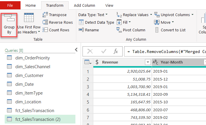
  1. Select the Columns for Grouping: In the Power Query editor, select the Year and Revenue columns in the fct_SalesTransaction query.
  2. Apply Group By: Go to Transform > Table > Group By. In the Group By dialog box, specify Year as the grouping column and set an aggregation function for Revenue, such as Sum, to calculate total revenue by year.
  3. Adjust Data Type: After grouping, change the data type of the resulting column to Currency – $ for consistency, particularly in financial data.
  4. Sort and Finalize: Sort the results by Month-Year in ascending order to maintain a chronological layout.

image68 image69

Excel: Free Masterclass​
Supercharge Your Skills For Free

20. Append vs. Merge Data

Append and Merge in Power Query are two methods of combining data, each designed for different types of data integration.

Append Data

The Append feature is useful for combining multiple datasets with the same structure, such as annual reports or monthly data files.

  1. Create Reference Queries for Each Year:
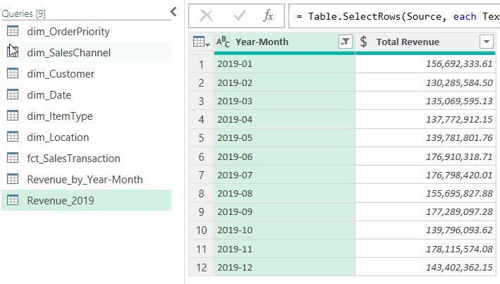
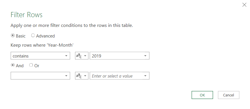
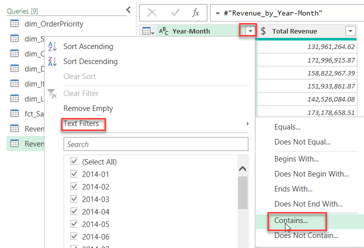
    • Start with the Revenue_by_Year-Month query and create a reference query for each year.
    • To create a reference query for 2019, apply a filter by selecting Year-Month > Text Filters > Contains > 2019. Repeat for 2020 and 2021.
  2. Rename Each Reference Query:
    • Rename each query to reflect the respective year (Revenue_2019, Revenue_2020, Revenue_2021).
  3. Combine Queries with Append:
    • Go to File > Combine > Append Queries as New.
    • In the Append Queries dialog, choose Three or more tables.
    • Select Revenue_2019, Revenue_2020, and Revenue_2021, then click Add.
  4. Finalizing the Append Query:
    • A new query, Append1, will be created.
    • Rename this query to App_Revenue_2019-2021.

This creates a single table containing data from all three years, stacking the rows vertically.
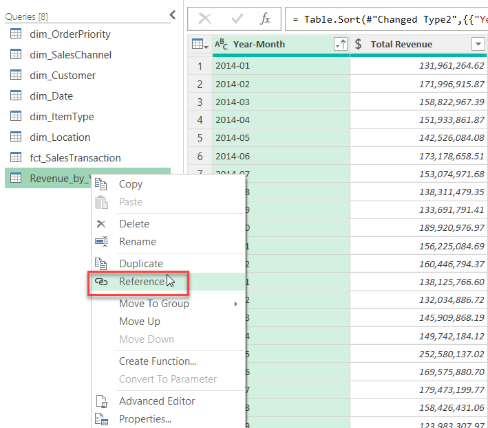
image53 image57 image56 image55 image54

Merge Data

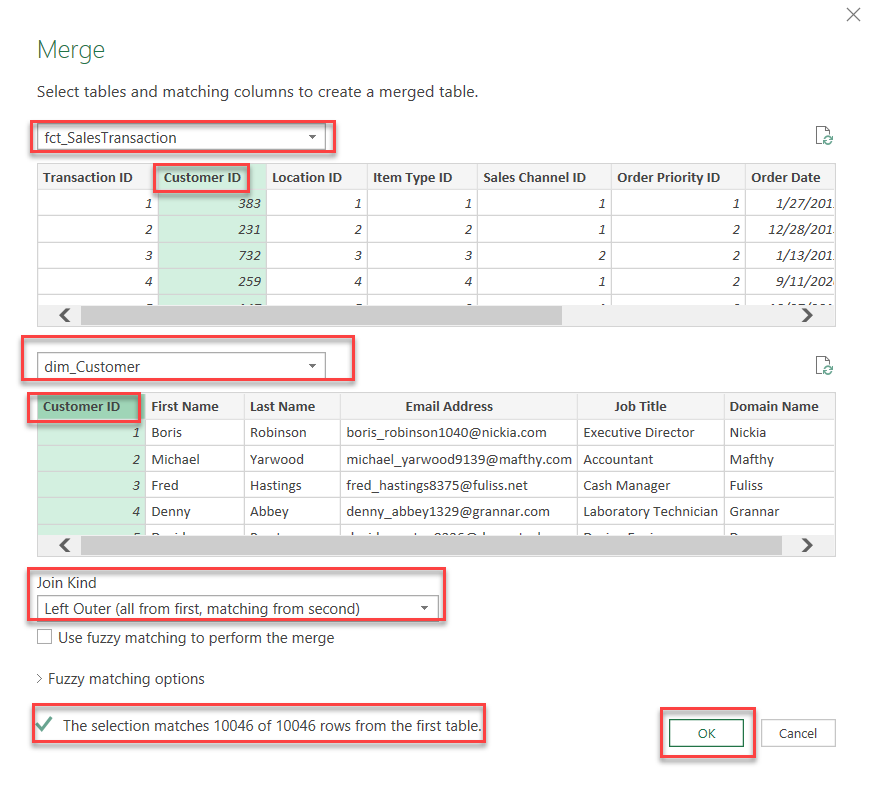
The Merge feature is used for joining tables with related information, similar to SQL joins. This process is helpful for combining two datasets with a common key field.

  1. Select Main Table for Merging:
    • Start with the fct_SalesTransaction query.
    • Go to Home > Combine > Merge Queries as New.
  2. Choose the Related Table and Join Type:
    • Select dim_Customer as the related table.
    • Choose Customer ID as the join key and select Left Outer Join to include all rows from fct_SalesTransaction.
  3. Confirm the Merge:
    • Click OK to apply the merge.
    • The merged query, Merge1, will display matched rows from dim_Customer.
  4. Add Specific Columns:
    • Expand dim_Customer and select columns like First Name and Last Name.
    • Rename the query to fct_SalesTransaction2, positioning First Name and Last Name next to Customer ID.

The Append operation stacks rows, while Merge joins tables based on a key column, allowing for flexible data analysis.

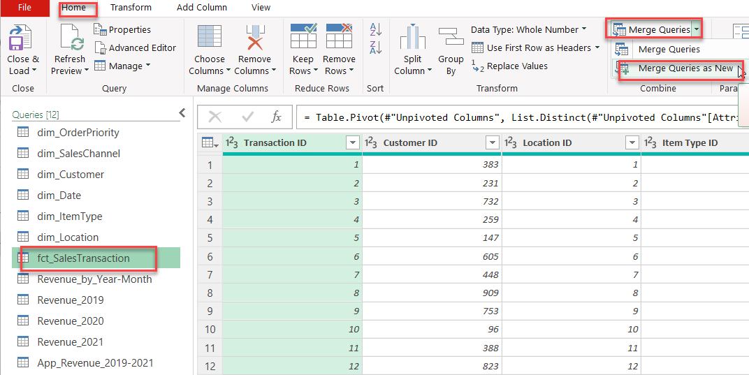
image87 image89 image91 image93

Excel: Free Masterclass​
Supercharge Your Skills For Free

Frequently Asked Questions

What is Power Query used for?

Power Query is a tool for extracting, transforming, and loading (ETL) data from various sources into Excel, making data management and analysis easier.

Can Power Query handle large datasets?

Yes, Power Query efficiently processes large datasets from multiple sources, allowing dynamic updates and seamless data transformations.

What types of files can be imported into Power Query?

Power Query can import data from various sources, including Excel files, text files, CSVs, databases (like Access), and web data.

Conclusion

Power Query is a powerful ETL tool that revolutionizes data management within Excel, making it easier to extract, transform, and load data from various sources. By using Power Query features like importing, transforming, unpivoting, and merging data, you can enhance data accuracy and efficiency for analysis. Mastering these tools helps simplify complex data workflows, creating a streamlined, efficient process.

Facebook
X
LinkedIn
Pinterest
Email
Table of Contents

Office Tech Skill is a premier educational platform focused on Microsoft Office, providing professionals with the tools needed to thrive in the ever-evolving tech landscape.

© 2024 Office Tech Skill. All rights reserved